Download presentation
Presentation is loading. Please wait.

1
Dr. Guy Tel-Zur Computational Physics Differential Equations Autumn Colors, by Bobby Mikul, http://www.publicdomainpictures.netBobby Mikul Autumn Colors, by Bobby Mikul, http://www.publicdomainpictures.netBobby Mikul Version 10-11-2010 18:30

2
Agenda MHJ Chapter 13 & Koonin Chapter 2 How to solve ODE using Matlab Scilab

3
Topics Defining the scope of the discussion Simple methods Multi-Step methods Runge-Kutta Case Studies - Pendulum

4
The scope of the discussion For a higher order ODE a set of coupled 1 st order equations:

5
Simple methods Euler method: Integration using higher order accuracy: Taylor series expansion:

6
Local error! Better than Euler’s method but useful only when it is easy to differentiate f(x,y)
")
7
Example Let’s solve:

9
FORTRAN code

10
Multi-Step methods

11
Adams-Bashforth 2 steps: 4 steps:

12
(So far) Explicit methods Future = Function(Present && Past) Implicit methods Future = Function(Future && Present && Past)
 Explicit methods Future = Function(Present && Past) Implicit methods Future = Function(Future && Present && Past)")
13
Let’s calculate dy/dx at a mid way between lattice points: Rearrange: This is a recursion relation! Let’s replace:

14
A simplification occurs if f(x,y)=y*g(x), then the recursion equation becomes: An example, suppose g(x)=-x y n+1 =(1-x n h/2)/(1+x n+1 h/2)y n This can be easily calculated, for example: Calculate y(x=1) for h=0.5 X0=0, y(0)=1 X1=0.5, y(0.5)=? x2=1.0, y(1.0)=?
= .")
15
The solution:

16
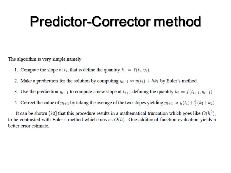
Predictor-Corrector method

18
Runge-Kutta

21
Proceed to: Physics examples: Ideal harmonic oscillator – section 13.6.1

22
Physics Project – The pendulum, 13.7 I use a modified the C++ code from: http://www.fys.uio.no/compphys/cp/programs/FYS3150/chapter13/cpp/program2.cpp fout.close fout.close() Demo on folder: C:\Users\telzur\Documents\BGU\Teaching\ComputationalPhysics\2011A\Lectures\05\CPP
 Demo on folder: C:\Users\telzur\Documents\BGU\Teaching\ComputationalPhysics\2011A\Lectures\05\CPP")
23
ODEs in Matlab function dydt = odefun(t,y) a=0.001; b=1.0; dydt -=b*t*sin(t)+a*t*t; function dydt = odefun(t,y) a=0.001; b=1.0; dydt -=b*t*sin(t)+a*t*t; Usage: [t1, y1]=ode23(@odefun,[0 100],0); Plot(t1,y1,’r’); hold on plot(t2,y2,’b’); hold off Usage: [t1, y1]=ode23(@odefun,[0 100],0); Plot(t1,y1,’r’); hold on plot(t2,y2,’b’); hold off Demo folder: Users\telzur\Documents\BGU\Teaching\ComputationalPhysics\2011A\Lectures\05\Matlab
![ODEs in Matlab function dydt = odefun(t,y) a=0.001; b=1.0; dydt -=b*t*sin(t)+a*t*t; function dydt = odefun(t,y) a=0.001; b=1.0; dydt -=b*t*sin(t)+a*t*t; Usage: [t1, 100],0); Plot(t1,y1,’r’); hold on plot(t2,y2,’b’); hold off Usage: [t1, 100],0); Plot(t1,y1,’r’); hold on plot(t2,y2,’b’); hold off Demo folder: Users\telzur\Documents\BGU\Teaching\ComputationalPhysics\2011A\Lectures\05\Matlab](http://images.slideplayer.com/11/3271114/slides/slide_23.jpg "ODEs in Matlab function dydt = odefun(t,y) a=0.001; b=1.0; dydt -=b*t*sin(t)+a*t*t; function dydt = odefun(t,y) a=0.001; b=1.0; dydt -=b*t*sin(t)+a*t*t; Usage: [t1, 100],0); Plot(t1,y1,’r’); hold on plot(t2,y2,’b’); hold off Usage: [t1, 100],0); Plot(t1,y1,’r’); hold on plot(t2,y2,’b’); hold off Demo folder: Users\telzur\Documents\BGU\Teaching\ComputationalPhysics\2011A\Lectures\05\Matlab")
24
Output

25
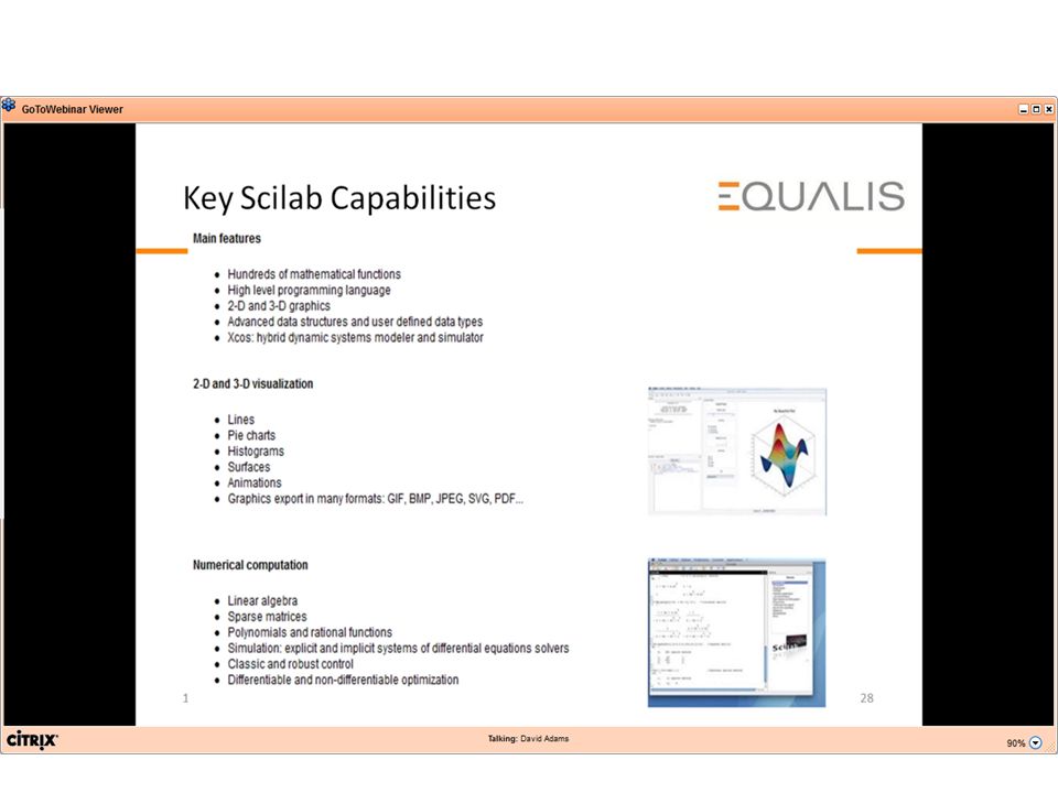
http://www.scilab.org

30
Parallel tools for Multi-Core and Distributed Parallel Computing

31
In preparation Parallel execution A new function (parallel_run) allows parallel computations and leverages multicore architectures and their capacities. Parallel execution A new function (parallel_run) allows parallel computations and leverages multicore architectures and their capacities.
 allows parallel computations and leverages multicore architectures and their capacities..")
37
Xcos demo

Similar presentations


 with the.>")
 Lecture 28-36 KFUPM Read 25.1-25.4, 26-2, 27-1 CISE301_Topic8L8&9 KFUPM.>")

 Pertemuan 12 Matakuliah: METODE NUMERIK I Tahun: 2008.>")


 1 1 Besides the main textbook, also see Ref.: “Applied.>")

 Lecture 28-36 KFUPM (Term 101) Section 04 Read 25.1-25.4, 26-2,>")