1. Sediment Quality Assessment and New York City Watersheds
Stephen Lewandowski
Major, United States Army
NYC Watershed/Tifft
Science & Technical Symposium
September 19, 2013
West Point, New York
Session XIV: Supply Protection (Location: Bradley South)
3:00 pm–3:30 pm
Sediments represent an important and dynamic compartment in aquatic ecosystems due to their ability to
serve as a sink of many chemical contaminants. However, there is currently no single recommended sediment
regulatory framework available. This study reviews existing sediment quality guideline (SQG) approaches
for their application to watershed protection and examines US EPA National Sediment Inventory (NSI) data
from the Catskill/Delaware and Croton watersheds. Key findings from the NSI analysis will be presented.

2. Importance of Sediment Quality
AGENDA
Importance of Sediment Quality
Overview of Sediment Quality Guidelines (SQGs) in New York
U.S. EPA National Sediment Inventory Data for Catskill/Delaware watershed
This presentation is organized into 3 primary parts:
- The importance of assessing sediment quality as part of a comprehensive ecosystem survey
Provide background on the guidelines used in New York state and the technical basis used for derivation
Investigate what the EPA NSI can tell us about the C-D watershed

3. Sediment Quality Introduction
Serve as “sink” for many chemicals
Ecology and human health effects
Sediment is comprised of all detrital, inorganic, or organic particles eventually settling on the bottom of a body of water (Power and Chapman 1992).

4. Sediment Processes
Figure 2.2. Sediment processes affecting the distribution and form of
contaminants. CA EPA, July 18, 2008
Sediment is a dynamic, complex material that plays an important role in aquatic ecosystems and provides habitat from a highly diverse community of organisms. Sediment-dwelling organisms range from microscopic bacteria and protozoans to large fish, amphibians, and reptiles that seek shelter and forage on the bottom, and may also hibernate there. Any and all of these organisms can potentially be put at risk from chemical contaminants in sediment, as well as wildlife that consume fish and invertebrates from the water body.
Sediment comes in a large range of sizes.
In flowing waters, streams and rivers, sediment is always on the move.
Sediments at the bottom of lakes and ponds are considerably different than sediments in streams.
Lakes can be described in terms of their trophic status, where trophy refers to the rate at which organic material is supplied by or to the lake per unit time
Because sediment is such a complex material, it has a much more complex effect on contaminants that can cause toxicity. Sediment characteristics such as pH, cation exchange capacity (CEC), redox potential, oxic state, composition of the sediment (e.g., sand, clay, silt), amount and type of clay present (e.g., kaolin, bentonite, montmorillonite, etc.), grain size, pore size, the nature and volume of organic carbon present, and the presence of sulfides, nitrates, carbonates, and other organic and inorganic substances, can alter the chemical and biological activity of contaminants. There can be a high degree of variability in the concentration of a contaminant that causes toxicity in different sediments, and no single concentration of a contaminant in sediment can accurately represent a threshold of toxicity for benthic organisms in all sediments.
Reduction potential (also known as redox potential, oxidation / reduction potential, ORP, pE, ε, or ) is a measure of the tendency of a chemical species to acquire electrons and thereby be reduced
Sediment processes affecting the distribution and form of contaminants (CA EPA)

5. Exposure Pathways
accessed 28 Aug 13

6. Sources and Receptors
Figure 2.1. Principal sources, fates, and effects of sediment contaminants
in enclosed bays and estuaries. Adapted from Brides et al
CA EPA, July 18, 2008
Sources, fates, and effects of sediment contaminants (CA EPA)

7. Sampling is Hard Work!

8. Equilibrium Partitioning (EqP)
NY State Approaches
Equilibrium Partitioning (EqP)
Consensus-based Sediment Quality Guidelines (freshwater sediments)
Effects Range Low (ERL)/ Effects Range Medium (ELM) (marine/estuarine sediments)
Image: USEPA, Procedures for the Derivation of Equilibrium Partitioning Sediment Benchmarks (ESBs)
for the Protection of Benthic Organisms: Endrin
Numerous efforts to develop suitable sediment quality guidelines for classifying sediment as toxic (contaminated) or non-toxic (relatively uncontaminated) have been published in the scientific literature.
In order to best protect aquatic resources, the scientific literature was reviewed to identify existing sets of candidate sediment guidelines for use in New York State as numeric Sediment Guidance Values (SGVs), for the purpose of classifying sediments with respect to their potential for adverse impacts. As a result of that review, three methods were chosen for establishing New York State SGVs: equilibrium partitioning (EqP); consensus-based sediment quality guidelines for freshwater sediments (MacDonald, et al. 2000); and ERL/ERMs for marine/estuarine sediments (Long, et al. 1995).

9. Equilibrium Partitioning
Mechanistic: uses fundamental knowledge of the interactions between process variables to define the model structure
Basis: non-polar organic contaminants will partition between sediment pore water and the organic carbon content of sediment in a constant ratio
ratio of the concentration in water to the concentration in organic carbon is termed the organic carbon partition coefficient (KOC)
Limitations:
does not consider the antagonistic, additive or synergistic effects of other sediment contaminants
does not account for bioaccumulation and trophic transfer to aquatic life, wildlife or humans
Equilibrium partitioning is a mechanistic methodology for deriving SGVs for nonpolar organic contaminants from their corresponding ambient water quality standards or guidance values (AWQS/GVs) and their affinity to adsorb to organic carbon in sediment.
EqP theory holds that a nonionic chemical in sediment partitions between sediment organic
carbon, interstitial (pore) water and benthic organisms. At equilibrium, if the concentration in
any one phase is known, then the concentrations in the others can be predicted. The ratio of the
concentration in water to the concentration in organic carbon is termed the organic carbon
partition coefficient (KOC), which is a constant for each chemical. The ESB Technical Basis
Document (U.S. EPA, 2003a) demonstrates that biological responses of benthic organisms to
nonionic organic chemicals in sediments are different across sediments when the sediment
concentrations are expressed on a dry weight basis, but similar when expressed on a ug chemical/g organic carbon basis (ug/g OC). Similar responses were also observed across sediments when interstitial water concentrations were used to normalize biological availability. The Technical Basis Document further demonstrates that if the effect concentration in water is known, the effect concentration in sediments on a ug/g OC basis can be accurately predicted by multiplying the effect concentration in water by the chemical’s KOC. .

10. Consensus-based Guidelines
Empirical: derived from field-collected data
Basis: relates measured concentrations of contaminants in sediments to observed biological effects
ERL – Effects Range Low: the 10th percentile concentration in a range of sediment concentrations for a given contaminant wherein adverse biological effects were observed
ERM – Effects Range Median: the 50th percentile concentration in a range of sediment concentrations for a given contaminant wherein adverse biological effects were observed
TEC – Threshold Effects Concentration : derived by taking the geometric mean of similar sediment quality guidelines for concentrations of contaminants that below which, no adverse impacts would be anticipated
PEC – Probable Effects Concentration: derived by taking the geometric mean of similar sediment quality guidelines for concentrations of contaminants that above which, adverse impacts would be expected to occur frequently
ERL: Effects Range Low; ERM: Effects Range Medium
TEL: Threshold effects (5oth %ile no effects/ 15th effects); PEL: Probable effects (80th/50th)
The major limitation of LRM and other empirical approaches is that they classify individual chemicals independent of the other constituents that make up the sample and are therefore restricted in their ability to describe cause-and-effect and additive relationships

11. Sediment Classification
Class A - No Appreciable Contamination (no toxicity to aquatic life)
EqP: chronic AWQS/GVs
empirically-based: threshold effects concentration (TEC) or Effects Range Low (ERL)
Class B - Moderate Contamination (potential for chronic toxicity to aquatic life)
contaminant concentrations found between the threshold concentrations which define Class A and Class C
Class C - High Contamination (potential for acute toxicity to aquatic life)
EqP: acute AWQS/GVs
empirically-based: probable effects concentration (PEC) or Effects Range Medium (ERM)
There is high variability in the concentration of contaminants in sediment that cause toxicity. When reviewing studies that compare sediment bulk chemistry data and toxicity, there is a typical pattern across the concentration gradient. At low concentrations, there is a range where toxicity does not occur. At higher concentrations, there is a range where toxicity consistently occurs. In between, concentration and toxicity results are mixed. A given contaminant concentration might be toxic in one sediment sample but not in another. Within this range, toxicity cannot be reliably predicted simply from the contaminant concentration in sediment.

12. Multiple Lines of Evidence
Sediment quality triad (SQT) decision matrix
Chemical contamination
Laboratory toxicity
Benthos alteration
Possible conclusions +
Strong evidence for pollution-induced degradation; management actions required. -
Strong evidence against pollution-induced degradation; no management actions required.
Contaminants are not bioavailable; no management actions required.
Unmeasured contaminant(s) or condition(s) have the potential to cause degradation; no immediate management actions required.
Benthos alteration is not due to toxic contamination; no toxic management actions required.
Toxic contaminants are bioavailable but in situ effects are not demonstrable – need to determine reason(s) for sediment toxicity.
Unmeasured toxic contaminants are causing degradation – need to determine reasons for sediment toxicity and benthos alteration.
Contaminants are not bioavailable; alteration not due to toxic chemicals – need to determine reason(s) for benthos alteration.
A weight of evidence approach can be very beneficial when evaluating risks from sediment contamination and is likely to result in more defensible sediment assessments. Any meaningful assessment of sediment quality needs to involve consideration of multiple lines of evidence, typically from sediment chemistry, ecotoxicology, and benthic ecology
Sediment guidance values are primarily useful as the initial step in a hierarchal approach for addressing a sediment contamination problem. They are a conservative tool for making an initial assessment of the potential risks that might be associated with contaminants in a sediment sample.
The best-known example of a weight of evidence approach is the sediment quality triad (SQT) (Long and Chapman 1985; Chapman 1990). The SQT uses the results of three different types of sediment evaluations to ascertain risk: bulk sediment dry weight concentrations, sediment toxicity tests, and benthic community analyses
A benthic community analysis, or macrobenthic community analysis, is a study that examines the characteristics of the benthic community that inhabits a possibly contaminated site. A benthic community analysis requires the use of a reference site or sites wherein the physical and chemical characteristics of the sediment are comparable to those at the site being evaluated. Several different biometrics have been proposed for evaluating the health of the resident benthic community. Typical metrics include species abundance and richness.

13. Multiple Lines of Evidence (California)
Multiple Lines of Evidence (CA Approach)
Steven M. Bay and Stephen B. Weisberg, A framework for interpreting sediment quality triad data
-Address two key elements of a risk assessment paradigm: 1) Is there biological degradation at the site?
and 2) Is chemical exposure at the site high enough to potentially result in an adverse biological response?
A combination of four benthic community condition indices was used to determine the magnitude of disturbance to the benthos at each site.
Steven M. Bay and Stephen B. Weisberg, A framework for interpreting sediment quality triad data

14. MLOE (CA Approach)
Multiple Lines of Evidence (CA Approach), Steven M. Bay and Stephen B. Weisberg, A framework for interpreting sediment quality triad data
Steven M. Bay and Stephen B. Weisberg, A framework for interpreting sediment quality triad data

15. National Sediments Inventory
Data from
More than 50,000 stations
~ 4.6 million observations
River, lake, ocean, estuary sediments
Mandated by Water Resources
Development Act of 1992
EPA reports to Congress: 1998 and 2004
The NSI is an extensive database that contains approximately 4.6 million observations compiled from multiple studies between 1980 and 1999 from more than 50,000 stations throughout the United States. The EPA developed the NSI as part of a national sediment quality survey directed by the Water Resources Development Act (WRDA) of 1992 (EPA 2004). The NSI includes data on surface and subsurface sediment chemistry, fish tissue residue, and bioassay toxicity results collected between 1980 and 1999, of which this study utilizes its surface chemistry and bioassay components. NSI sample stations represent 5,695 river reaches with sediment samples from river, lake, ocean, and estuary bottoms, representing both freshwater and marine environments.

16. Bioassay Toxicity Tests
EPA: significant toxicity  20% difference in survival from control
Medium: Bulk sediment
Endpoint: Percent mortality
Images:
Ampelisca abdita (marine amphipod)

17. Human Health Screening Values (SV)a for Interpreting National Lake Fish Tissue Study Predator Results
The National Study of Chemical Residues in Lake Fish Tissue
EPA, September 2009
The National Study of Chemical Residues in Lake Fish Tissue (EPA, 2009)

18. 50,778 stations NSI Samples 50,778 stations
14,531 bioassay observations
50,778 stations

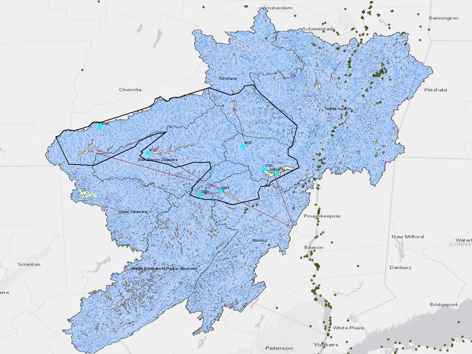
19. n = 2,239 (NY) 6 C-D subbasins (HU-8), n = 278 NSI Stations in NY
Blue: 6 C-D subbasins (HU-8): 278 of 2239 stations
n = 2,239 (NY)
6 C-D subbasins (HU-8), n = 278

20. Stations in C-D Watershed Boundary, n = 9
Schoharie Reservoir 2
Pepacton Reservoir 3
Cannonsville Reservoir
Ashokan Reservoir
Roundout
Reservoir
Neversink
Reservoir
Catskill Aqueduct
Delaware Aqueduct
Stations in C-D Watershed Boundary, n = 9

21. Fish Tissue Species SMB: smallmouth bass BT: brown trout
Majority of tissue samples collected in 1998.
SMB: smallmouth bass
BT: brown trout
WS: white sucker
RB: rock bass

22. % lakes above in EPA study
health endpoint
SV fish tissue conc
units
% lakes above in EPA study
Mean
(ppb)
Confidence Level(95.0%)
Count
Mercury
noncancer
300
ppb
48.8
484.29
43.55
217
Chlordane
cancer 67
0.3 ND 19
DDT 69
1.7
pp-DDE
5.37
1.07
pp-DDT
12.79
5.69
pp-DDD
Mercury 146 samples at or above SV
The National Study of Chemical Residues in Lake Fish Tissue (EPA-823-R ), U.S. Environmental Protection Agency, September 2009.

23. Tissue concentrations (ppb)
Units for PCBs wrong?

24. Mercury Tissue Histogram
Hg Screening value = 300 ppb

25. Mercury Tissue by Station
vic. Esopus Creek (Catskill)
Roundout (Delaware)
Pepacton (Delaware)
Neversink (Delaware)
Ashokan (Delaware)
The distribution of mercury (Hg) and sites of greatest Hg methylation are poorly understood in Catskill Mountain watersheds. Although concentrations of Hg in the water column are low, high concentrations of Hg in smallmouth bass and walleye have led to consumption advisories in most large New York City reservoirs in the Catskill Mountains. Mercury in natural waters can exist in many forms, including gaseous elemental mercury (Hg0), dissolved and particulate inorganic forms (Hg(II)), and dissolved and particulate methylmercury (MeHg). Most Hg in living organisms is MeHg, a highly neurotoxic form that bioaccumulates in aquatic food webs. The production of MeHg by methylation of inorganic Hg in the environment is a key process affecting the quantity of MeHg accumulated in fish. Small quantities of MeHg in the diet can adversely affect wildlife and humans, which are exposed to MeHg almost entirely through the consumption of fish.
The Neversink watershed is a high relief, forested ecosystem that supplies part of New York City's drinking water supply. This watershed is in the general vicinity of some of the highest suspected atmospheric Hg deposition zones in the coterminous US, and as such the Hg problem here is likely not limited to the current supply of Hg in the watershed.
Ashokan (Delaware)
Screening value = 300 ppb

26. Sediments are an important component of watershed ecosystems
Summary
Sediments are an important component of watershed ecosystems
New York State applies screening guidelines derived from both mechanistic and empirical models to classify contamination and potential for toxicity
National sediments database is useful for a historical perspective on contaminants and development of guidelines
Image:

27. Environmental Program (Dr. Marie Johnson)
Acknowledgements
United States Military Academy, Dept. of Geography & Environmental Engineering
Environmental Program (Dr. Marie Johnson)
Geospatial Lab (COL Michael Hendricks)
Harvard School of Public Health
Professor Jim Shine
Professors Francine Laden and Bob Herrick
Image:

28. References
Screening and Assessment of Contaminated Sediment. New York State Department of Environmental Conservation, Division of Fish, Wildlife and Marine Resources, Bureau of Habitat, January 24, 2013 (Draft Version 4.0)
Technical Guidance for Screening Contaminated Sediments. New York State Department of Environmental Conservation, Division of Fish, Wildlife and Marine Resources, January 25, 1999.
The National Study of Chemical Residues in Lake Fish Tissue (EPA-823-R ), U.S. Environmental Protection Agency, September 2009.
The Incidence and Severity of Sediment Contamination in Surface Waters of the United States, U.S. Environmental Protection Agency, Office of Science and Technology, 1997.
The Incidence and Severity of Sediment Contamination in Surface Waters of the United States, National Sediment Quality Survey: Second Edition, US EPA, 2004.

29. BACK-UP
Back-Up Slides
HSPH Practicum Multivariable Regression Sediment-Toxicity Model
Additional GIS Maps
C-D Fish Tissue Data Analysis

30. Site on fish gill (or other receptor) is a ligand too
Biotic Ligand Model
Site on fish gill (or other receptor) is a ligand too
The biotic ligand model is actually a water quality model, used to predict the toxicity of metals in water (Paquin, et al. 2002). The most toxic form of a metal in water is the divalent metal ion (M++) or ionic hydroxide species (MOH+). Various organic and inorganic ligands in water can bind ionic species of metal, and limit their availability for uptake by organisms. The model uses a number of water quality characteristics (temperature, pH, alkalinity, and concentration of dissolved organic carbon (DOC), major cations (Ca, Mg, Na, K), major anions (SO4, Cl, S)) to predict the availability and toxicity of the metal. The biotic ligand model is the basis for the U.S. EPA water quality criteria for copper (U.S. EPA 2007).
Shine (2010)
Gill is primary site of toxic action for most metals, especially
for freshwater organisms and acute toxicity

31. Mercury Cycle

32. Arsenic Redox Conditions
Shine (2010)
Shine (2010)

33. Data Analysis Binary dependant variable (toxicity)
Continuous predictor variables (concentrations)
Pr(tox=1) = F(β0 + β1chem1 + β2chem2 + β3chem3… βnchemn
We built the multivariable logistic regression model using toxicity as a binary dependant variable and chemical concentrations as continuous predictor variables. The model is fit by the equation : Pr(tox=1) = F(β0 + β1chem1 + β2chem2 + β3chem3… βnchemn.
 Station
Toxic Effect
Metal 1
Metal 2
Metal 3
PAHs
PCBs
DDT
TOC A 1
conc.
percentage B C D

34. Surface Chemistry Dataset
Data Management
Bioassay Dataset
B1. Include all species or sort
B2. Compress from sample-level to station level
B3. Threshold for station tox based on mean sample tox
B4. Merge with surface chemistry dataset by station
Surface Chemistry Dataset
C1. Select analytes to retain
C2. Drop duplicate entries
C4. Merge with bioassay dataset by station
C3. Compress to station-level with mean sample concentrations
Paired Dataset
P1. Drop unmatched observations
P2. Reshape data from long to wide
P3. Remove observations with missing chemical concentrations
P4. Apply MLRM

35. Results Model 1 2 3 4 Description
All bioassay species, 23 chemicals + 10th root TOC
Ampelisca abdita, 23 chemicals + 10th root TOC
Ampelisca abdita, sigma PAH + 11 chemicals + 10th root TOC
Stepwise backward, Model 3: As, Cd, Cu, Hg, pyrene n
1,789
1,557
Significant positive variables (α=0.05)
Cu, Hg, 10th root TOC
Cd, Cu, Ni
Cd, Cu, Hg
Significant negative variables (α=0.05)
acenaphthylene, dibenz(a,h)anthracene, napthalene, PCBs As
BIC
-11,024
-9,687
-9,756
-9,809
HL GOF χ2 (8),
(p-value)
15.41 (0.052)
4.15 (0.843)
4.72 (0.787)
5.59 (0.6925)
Area under ROC curve
0.72
0.695
0.696
0.678
Toxicity distribution (% stations coded as toxic)
51.7
26.1
BIC: Bayesian Information Criterion (more negative values indicate better model fit)
HL GOF: Hosmer-Lemeshow goodness-of-fit test (small p-values indicate a lack of fit)
ROC: receiver operating characteristic, plot of sensitivity vs. false positive rate, closer to 1 indicates better accuracy

36. Model Evaluation Bayesian Information Criterion (BIC)
more negative values indicate better model fit
Hosmer-Lemeshow goodness-of-fit test
small p-values indicate a lack of fit
Receiver operating characteristic (ROC)
plot of sensitivity vs. false positive rate
closer to 1 indicates better accuracy

37. Selected Model
DV: Ampelisca abdita toxicity IVs: ∑PAH + 11 chemicals + 10th root TOC
 Variable
Odds Ratio
95% Conf. Interval
∑ PAH#
1.01
1.00
1.03
PCBs
0.96
0.51
1.82
DDT##
2.47
0.05
131.74
root10_TOC
0.25
0.02
2.71
Metals
ARSENIC**
0.93
0.91
CADMIUM*
1.44
1.11
1.87
CHROMIUM
0.99
COPPER*
1.02
LEAD
MERCURY
1.30
0.94
1.78
NICKEL*
SILVER
0.98
0.81
1.19
ZINC
# PAHs
acenapththene
anthracene
benzo(a)anthracene
dibenz(a,h)anthracene
benzo(a)pyrene
chrysene
fluoranthene
indeno(1,2,3-c,d)pyrene
naphthalene
phenanthrene
pyrene
## DDT Isomers
DDD, p, p’
DDE, p, p’
DDT, p, p’
Ampelisca abdita, sigma PAH + 11 chemicals + 10th root TOC
* Significant positive effect at α=0.05
** Significant negative effect at α=0.05

38. Discussion Decent overall model fit and predictive value
High specificity, but low sensitivity
Scientific plausibility
Cadmium, copper, nickel as positive indicators
Arsenic as a negative indicator
Species could be adaptive to As in seawater  convert to arsenobetaine
Suggestive of oxidized conditions: As(V) vs As (III)
Competition for binding sites on sediment particles and biotic ligand receptors
Hg, Pb not significant  may be tightly bound with low bioavailability
Large standard error for DDT

39. Chemical Analysis  Exposure Misclassification
Limitations
Impacts confidence and generalizablility
Chemical Analysis  Exposure Misclassification
Different methods by study and over time from
Handling of detection limits/ low concentrations
Bioassay
Species appropriate
Consistent methods and endpoint determination (EPA toxicity classification)
Data set
Spatial resolution: sample vs. station identification
Data input errors
Model: limited in number of parameters; trade-offs in selection of species and chemical predictors; care not to over-fit model
 Maintain large n with a complete representation of chemicals

40. Conclusions
Able to develop a reasonable MLRM with decent goodness of fit and predictive value
for A. abdita toxic effects from surface sediment chemical concentrations
Big limitations and uncertainty from the data set structure, chemical analysis, bioassays and the statistical model reduce overall confidence
Methodology adds value for investigating data and physical and chemical relationships
Multiple lines of evidence with knowledge of local area should be examined to assess sediment quality

41. Predictive Variable Selection41
Chemical
class
chemcode
freq
DDE, p,p'
DDT
PP_DDE
22,771
DDT, p,p'
PP_DDT
22,330
DDD, p,p'
PP_DDD
22,103
Dieldrin
Insecticide
DIELDRIN
34,007
Lead
Metal
LEAD
58,389
Copper
COPPER
56,496
Cadmium
CADMIUM
55,665
Zinc
ZINC
54,846
Mercury
MERCURY
53,069
Chromium, total
CHROMIUM
52,657
Arsenic
ARSENIC
47,845
Nickel
NICKEL
45,551
Silver
SILVER
29,850
Antimony
ANTIMONY
16,535
Fluoranthene
PAH
FLUORANTHN
21,319
Pyrene
PYRENE
21,121
Chrysene
CHRYSENE
20,885
Phenanthrene
PHENANTHRN
20,586
Anthracene
ANTHRACENE
20,205
Acenaphthene
ACENAPTHEN
20,075
Naphthalene
NAPTHALENE
20,014
Benzo(a)anthracene
BAA
19,760
Benzo(g,h,i)perylene
BGHIP
19,513
Benzo(a)pyrene
BAP
19,465
Fluorene
FLUORENE
19,213
Acenaphthylene
ACENAPTYLE
19,203
Benzo(k)fluoranthene
BKF
14,397
Benzo(b)fluoranthene
BBF
14,383
Methylnaphthalene, 2
METHNAP_2
12,977
Perylene
PERYLENE
182
Methylnaphthalene, 1
METHNAP_1
141
Methylphenanthrene, 1
METPHENAN1
117
Dibenz(a,h)anthracene
unk
Dimethylnaphthalene, 2,6
Indeno(1,2,3-c,d)pyrene
Polychlorinated biphenyls
PCB
PCB_SUM
31,738
Biphenyl
BIPHENYL
151

42. Chemistry: Inorganic
Metals As Cd Cr Cu Pb Hg Ni Zn

43. Chemistry: Organic Polycyclic aromatic hydrocarbons (∑)
Acenapththene
Anthracene
Benzo(a)anthracene
Benzo(a)pyrene
Fluoranthene
Naphthalene
Phenanthrene
Pyrene
Organochlorines
Polychlorinated biphenyls (PCBs, total)
DDT (∑)
DDD, p, p’
DDE, p, p’
DDT, p, p’

46. C-D Watershed Layer

48. NSI Stations

49. NSI Fields

50. 2 metals (mercury and 5 forms of arsenic) 17 dioxins and furans
> summary(smptiss9)
X siteid studyid stationid sampleid fieldrep labrep sampdate species
Min. : Min. : Min. : AS001 :59 A0 : 8 #: #:236 Min. : SMB :51
1st Qu.: st Qu.: st Qu.: AS002 :57 A1 : st Qu.: BT :40
Median : Median : Median : RR001 :50 A2 : Median : WS :29
Mean : Mean : Mean : NV001 :47 A3 : Mean : RB :27
3rd Qu.: rd Qu.: rd Qu.: TR001 :12 A4 : rd Qu.: YP :16
Max. : Max. : Max. : HE001 : 7 A5 : Max. : RT :13
(Other): 4 (Other): (Other):60
tissue noincomp length weight sex pctlipid exsampid
HV: 22 Min. : Min. : Min. : F: 1 Min. : Mode:logical
SF: st Qu.: st Qu.: st Qu.: M: st Qu.: NA's:236
WH: 7 Median : Median : Median : U:233 Median :2.850
Mean : Mean : Mean : Mean :2.968
3rd Qu.: rd Qu.: rd Qu.: rd Qu.:3.480
Max. : Max. : Max. : Max. :6.860
NA's :215
SPECIES
Value # of Cases % Cumulative %
1 BB
2 BDACE
3 BLC
4 BRT
5 BT
6 CARP
7 CCHUB
8 CMSH
9 LLS
10 LMB
11 LT
12 PICK
13 RB
14 RT
15 SMB
16 WEYE
17 WS
18 YB
19 YP
Case Summary
Valid Missing Total
# of cases
$tissue
Frequencies
Value # of Cases % Cumulative %
1 HV
2 SF
3 WH
Case Summary
Valid Missing Total
# of cases
Tissue residue data include detailed analytical results, analyte sampled, species,
sex, tissue type, length, qualifier for concentration, field and laboratory replication identifier, and
weight.
The laboratories under contract to EPA analyzed the fish tissue samples for the following target chemicals:
  2 metals (mercury and 5 forms of arsenic)
 17 dioxins and furans
159 PCB congener measurements (representing results for 209 congeners)
 46 pesticides
 40 other semi-volatile organics (e.g., phenols)

51. > frequencies(smptiss9[c("stationid")] , r.digits = 1)
Frequencies
Value # of Cases % Cumulative %
1 AS
2 AS
3 HE
4 NV
5 PP
6 RR
7 TR
8 UE
SMB: small-mouth bass
BT: brown trout
WS: white sucker
RB: rock bass
YP: yellow perch
YB:
RT: rainbow trout

52. Recommended Target Species for Lakes and Reservoirs
The National Study of Chemical Residues in Lake Fish Tissue
EPA, September 2009
- The species is abundant and commonly consumed in the study area.
- It may potentially accumulate high concentrations of chemicals.
- The species is easy to identify, and it has a wide geographic distribution.
- Adult specimens are large enough to provide adequate tissue for analysis.

53. % lakes above in EPA study
health endpoint
SV fish tissue conc
units
% lakes above in EPA study
Mean
Standard Error
Standard Deviation
Minimum
Maximum
Count
Confidence Level(95.0%)
Mercury
noncancer
300
ppb
48.8
484.29
22.09
325.47
50.00
217.00
43.55
PCBs
cancer 12
16.8
538.98
204.00
19.00
Chlordane 67
0.3 ND
DDT 69
1.7
pp-DDE
5.37
0.51
2.22
2.00
12.00
1.07
pp-DDT
12.79
2.71
11.80
43.00
5.69
pp-DDD
Mercury 146 samples at or above SV