Download presentation
Presentation is loading. Please wait.

1
Overview of some tests Thomas INGICCO J.L.T. Géricault, Le Radeau de La Méduse J.L.T. Géricault, The Raft of The Medusa

2
Chi square test Aim: Comparison of observed effectives Oij to theoretical effectives Eij Are the lines and columns of a crossed table independant? Meaning that being part of the first variable has no influence on the modality of being part of the second variable.

3
Chi square test Aim: Comparison of observed effectives Oij to theoretical effectives Eij Are the lines and columns of a crossed table independant. Meaning that being part of the first variable has no influence on the modality of being part of the second variable. Measured variable: A qualitative variable with k classes

4
Chi square test Aim: Comparison of observed effectives Oij to theoretical effectives Eij Are the lines and columns of a crossed table independant. Meaning that being part of the first variable has no influence on the modality of being part of the second variable. Measured variable: A qualitative variable with k classes Conditions of utilization: The class of the variables must be exclusives Cochran’s rule must be respected: in each class Eij ≥ 5. But possiblity to have some classes with 1 ≤ Oij ≤ 5 if a minimum of 80% of the totality of the classes have Oij > 5

5
Chi square test Aim: Comparison of observed effectives Oij to theoretical effectives Eij Are the lines and columns of a crossed table independant. Meaning that being part of the first variable has no influence on the modality of being part of the second variable. Measured variable: A qualitative variable with k classes Conditions of utilization: The class of the variables must be exclusives Cochran’s rule must be respected: in each class Eij ≥ 5. But possiblity to have some classes with 1 ≤ Oij ≤ 5 if a minimum of 80% of the totality of the classes have Oij > 5 Test hypotheses: H0: π i = P théo i The theoretical proportions P théo i are the real proportions in the observed population H1 bilat : One at least of the theoretical proportions is not the real proportion in the observed population

6
Chi square test Aim: Comparison of observed effectives Oij to theoretical effectives Eij Are the lines and columns of a crossed table independant. Meaning that being part of the first variable has no influence on the modality of being part of the second variable. Measured variable: A qualitative variable with k classes Conditions of utilization: The class of the variables must be exclusives Cochran’s rule must be respected: in each class Eij ≥ 5. But possiblity to have some classes with 1 ≤ Oij ≤ 5 if a minimum of 80% of the totality of the classes have Oij > 5 Test hypotheses: H0: π i = P théo i The theoretical proportions P théo i are the real proportions in the observed population H1 bilat : One at least of the theoretical proportions is not the real proportion in the observed population The statistic is: In R:sum((Oij - Eij)^2/Eij)
^2/Eij).")
7
Chi square test In details: Ceram<-read.table("K:/Cours/Philippines/Statistics-210/Data/Ceramics.txt",header=TRUE)
")
8
Chi square test In details: Ceram<-read.table("K:/Cours/Philippines/Statistics-210/Data/Ceramics.txt",header=TRUE) obs1<-data.frame(Ceram[,10:11]) obs2<-na.omit(obs1) for(i in 1:length(obs2)){obs2[,i]<-factor(obs2[,i])} obs3<- table(obs2) addmargins(obs3)
![Chi square test In details: Ceram<-read.table( K:/Cours/Philippines/Statistics-210/Data/Ceramics.txt ,header=TRUE) obs1<-data.frame(Ceram[,10:11]) obs2<-na.omit(obs1) for(i in 1:length(obs2)){obs2[,i]<-factor(obs2[,i])} obs3<- table(obs2) addmargins(obs3)](http://images.slideplayer.com/11/3234051/slides/slide_8.jpg "Chi square test In details: Ceram<-read.table( K:/Cours/Philippines/Statistics-210/Data/Ceramics.txt ,header=TRUE) obs1<-data.frame(Ceram[,10:11]) obs2<-na.omit(obs1) for(i in 1:length(obs2)){obs2[,i]<-factor(obs2[,i])} obs3<- table(obs2) addmargins(obs3)")
9
Chi square test In details: Ceram<-read.table(i"K:/Cours/Philippines/Statistics-210/Data/Ceramics.txt",header=TRUE) obs1<-data.frame(Ceram[,10:11]) obs2<-na.omit(obs1) for(i in 1:length(obs2)){obs2[,i]<-factor(obs2[,i])} obs3<- table(obs2) addmargins(obs3) graphics.off() par(cex.lab=1.5, xpd=NA, font=2) mosaicplot(t(obs3), main=NULL, cex.axis=1.1)
![Chi square test In details: Ceram<-read.table(i K:/Cours/Philippines/Statistics-210/Data/Ceramics.txt ,header=TRUE) obs1<-data.frame(Ceram[,10:11]) obs2<-na.omit(obs1) for(i in 1:length(obs2)){obs2[,i]<-factor(obs2[,i])} obs3<- table(obs2) addmargins(obs3) graphics.off() par(cex.lab=1.5, xpd=NA, font=2) mosaicplot(t(obs3), main=NULL, cex.axis=1.1)](http://images.slideplayer.com/11/3234051/slides/slide_9.jpg "Chi square test In details: Ceram<-read.table(i K:/Cours/Philippines/Statistics-210/Data/Ceramics.txt ,header=TRUE) obs1<-data.frame(Ceram[,10:11]) obs2<-na.omit(obs1) for(i in 1:length(obs2)){obs2[,i]<-factor(obs2[,i])} obs3<- table(obs2) addmargins(obs3) graphics.off() par(cex.lab=1.5, xpd=NA, font=2) mosaicplot(t(obs3), main=NULL, cex.axis=1.1)")
10
Chi square test In details: Ceram<-read.table("K:/Cours/Philippines/Statistics-210/Data/Ceramics.txt",header=TRUE) obs1<-data.frame(Ceram[,10:11]) obs2<-na.omit(obs1) for(i in 1:length(obs2)){obs2[,i]<-factor(obs2[,i])} obs3<- table(obs2) addmargins(obs3) graphics.off() par(cex.lab=1.5, xpd=NA, font=2) mosaicplot(t(obs3), main=NULL, cex.axis=1.1) obs3theo<-suppressWarnings(chisq.test(obs3)$expected) addmargins(obs3theo) nij<-obs3 tij<-obs3theo chi2.calc<-sum((nij-tij)^2/tij) chi2.calc k<-dim(obs3)[1] c<-dim(obs3)[2] nu=(k-1)*(c-1) nu pchisq(chi2.calc, nu, lower.tail=FALSE)
![Chi square test In details: Ceram<-read.table( K:/Cours/Philippines/Statistics-210/Data/Ceramics.txt ,header=TRUE) obs1<-data.frame(Ceram[,10:11]) obs2<-na.omit(obs1) for(i in 1:length(obs2)){obs2[,i]<-factor(obs2[,i])} obs3<- table(obs2) addmargins(obs3) graphics.off() par(cex.lab=1.5, xpd=NA, font=2) mosaicplot(t(obs3), main=NULL, cex.axis=1.1) obs3theo<-suppressWarnings(chisq.test(obs3)$expected) addmargins(obs3theo) nij<-obs3 tij<-obs3theo chi2.calc<-sum((nij-tij)^2/tij) chi2.calc k<-dim(obs3)[1] c<-dim(obs3)[2] nu=(k-1)*(c-1) nu pchisq(chi2.calc, nu, lower.tail=FALSE)](http://images.slideplayer.com/11/3234051/slides/slide_10.jpg "Chi square test In details: Ceram<-read.table( K:/Cours/Philippines/Statistics-210/Data/Ceramics.txt ,header=TRUE) obs1<-data.frame(Ceram[,10:11]) obs2<-na.omit(obs1) for(i in 1:length(obs2)){obs2[,i]<-factor(obs2[,i])} obs3<- table(obs2) addmargins(obs3) graphics.off() par(cex.lab=1.5, xpd=NA, font=2) mosaicplot(t(obs3), main=NULL, cex.axis=1.1) obs3theo<-suppressWarnings(chisq.test(obs3)$expected) addmargins(obs3theo) nij<-obs3 tij<-obs3theo chi2.calc<-sum((nij-tij)^2/tij) chi2.calc k<-dim(obs3)[1] c<-dim(obs3)[2] nu=(k-1)*(c-1) nu pchisq(chi2.calc, nu, lower.tail=FALSE)")
11
Chi square test In details: # Test in R chisq.test(obs3)
")
12
Fisher test Aim: Comparison of observed effectives G & F (independance of 2 qualitatives variables) as observed proportions P G1/F1 and P G1/F2 (equality of the proportions)
 as observed proportions P G1/F1 and P G1/F2 (equality of the proportions)")
13
Fisher test Aim: Comparison of observed effectives G & F (independance of 2 qualitatives variables) as observed proportions P G1/F1 and P G1/F2 (equality of the proportions) Measured variable: Two qualitative variables F & G with 2 classes
 as observed proportions P G1/F1 and P G1/F2 (equality of the proportions) Measured variable: Two qualitative variables F & G with 2 classes")
14
Fisher test Aim: Comparison of observed effectives G & F (independance of 2 qualitatives variables) as observed proportions P G1/F1 and P G1/F2 (equality of the proportions) Measured variable: Two qualitative variables F & G with 2 classes Conditions of utilization: The class of the variables must be exclusives Qualitative variables are nominal
 as observed proportions P G1/F1 and P G1/F2 (equality of the proportions) Measured variable: Two qualitative variables F & G with 2 classes Conditions of utilization: The class of the variables must be exclusives Qualitative variables are nominal")
15
Fisher test Aim: Comparison of observed effectives G & F (independance of 2 qualitatives variables) as observed proportions P G1/F1 and P G1/F2 (equality of the proportions) Measured variable: Two qualitative variables F & G with 2 classes Conditions of utilization: The class of the variables must be exclusives Qualitative variables are nominal Test hypotheses: H0: π G1/F1 = π G1/F12 Proportions are identical i n the target population H1 bilat : π G1/F1 ≠ π G1/F12 Proportions are different in the target population H1 unilat right : π G1/F1 > π G1/F12 Proportion π G1/F1 is strictly superior to the target population H1 unilat left : π G1/F1 < π G1/F12 Proportion π G1/F1 is strictly inferior to the target population
 as observed proportions P G1/F1 and P G1/F2 (equality of the proportions) Measured variable: Two qualitative variables F & G with 2 classes Conditions of utilization: The class of the variables must be exclusives Qualitative variables are nominal Test hypotheses: H0: π G1/F1 = π G1/F12 Proportions are identical i n the target population H1 bilat : π G1/F1 ≠ π G1/F12 Proportions are different in the target population H1 unilat right : π G1/F1 > π G1/F12 Proportion π G1/F1 is strictly superior to the target population H1 unilat left : π G1/F1 < π G1/F12 Proportion π G1/F1 is strictly inferior to the target population")
16
Fisher test Aim: Comparison of observed effectives G & F (independance of 2 qualitatives variables) as observed proportions P G1/F1 and P G1/F2 (equality of the proportions) Measured variable: Two qualitative variables F & G with 2 classes Conditions of utilization: The class of the variables must be exclusives Qualitative variables are nominal Test hypotheses: H0: π G1/F1 = π G1/F12 Proportions are identical i n the target population H1 bilat : π G1/F1 ≠ π G1/F12 Proportions are different in the target population H1 unilat right : π G1/F1 > π G1/F12 Proportion π G1/F1 is strictly superior to the target population H1 unilat left : π G1/F1 < π G1/F12 Proportion π G1/F1 is strictly inferior to the target population The statistic is: In R:sum((Oij - Eij)^2/Eij)
 as observed proportions P G1/F1 and P G1/F2 (equality of the proportions) Measured variable: Two qualitative variables F & G with 2 classes Conditions of utilization: The class of the variables must be exclusives Qualitative variables are nominal Test hypotheses: H0: π G1/F1 = π G1/F12 Proportions are identical i n the target population H1 bilat : π G1/F1 ≠ π G1/F12 Proportions are different in the target population H1 unilat right : π G1/F1 > π G1/F12 Proportion π G1/F1 is strictly superior to the target population H1 unilat left : π G1/F1 < π G1/F12 Proportion π G1/F1 is strictly inferior to the target population The statistic is: In R:sum((Oij - Eij)^2/Eij)")
17
Fisher test In details:

18
Fisher test In details:

19
Fisher test In details:

20
Fisher test In details:

21
Fisher test In details: Ceram<-read.table("K:/Cours/Philippines/Statistics-210/Lecture- 4/Ceramics.txt",header=TRUE)
")
22
Fisher test In details: Ceram<-read.table("K:/Cours/Philippines/Statistics-210/Lecture- 4/Ceramics.txt",header=TRUE) obs1<-Ceram[,c(12,9)] obs2<-na.omit(obs1) for(i in 1:length(obs2)){obs2[,i]<-factor(obs2[,i])} obs3<- table(obs2) # obs3<-t(obs3) # obs4<-obs3 ; obs4[,1]<-obs3[,2] ; obs4[,2]<-obs3[,1] ; dimnames(obs4)[[2]][1] <- dimnames(obs3)[[2]][2] ; dimnames(obs4)[[2]][2] <- dimnames(obs3)[[2]][1] ; obs3<- obs4 addmargins(obs3)
![Fisher test In details: Ceram<-read.table( K:/Cours/Philippines/Statistics-210/Lecture- 4/Ceramics.txt ,header=TRUE) obs1<-Ceram[,c(12,9)] obs2<-na.omit(obs1) for(i in 1:length(obs2)){obs2[,i]<-factor(obs2[,i])} obs3<- table(obs2) # obs3<-t(obs3) # obs4<-obs3 ; obs4[,1]<-obs3[,2] ; obs4[,2]<-obs3[,1] ; dimnames(obs4)[[2]][1] <- dimnames(obs3)[[2]][2] ; dimnames(obs4)[[2]][2] <- dimnames(obs3)[[2]][1] ; obs3<- obs4 addmargins(obs3)](http://images.slideplayer.com/11/3234051/slides/slide_22.jpg "Fisher test In details: Ceram<-read.table( K:/Cours/Philippines/Statistics-210/Lecture- 4/Ceramics.txt ,header=TRUE) obs1<-Ceram[,c(12,9)] obs2<-na.omit(obs1) for(i in 1:length(obs2)){obs2[,i]<-factor(obs2[,i])} obs3<- table(obs2) # obs3<-t(obs3) # obs4<-obs3 ; obs4[,1]<-obs3[,2] ; obs4[,2]<-obs3[,1] ; dimnames(obs4)[[2]][1] <- dimnames(obs3)[[2]][2] ; dimnames(obs4)[[2]][2] <- dimnames(obs3)[[2]][1] ; obs3<- obs4 addmargins(obs3)")
23
In details: graphics.off() pG1.Fi<- obs3[, 1]/ margin.table(obs3, 1) par(mar=c(5.1, 5.1, 4.1, 2.1)) barplot(pG1.Fi, xlab = paste(labels(dimnames(obs3))[2], " / ", labels(dimnames(obs3))[1]), xaxt = "n", ylab="Proportion", ylim=range(0, max(pG1.Fi)+ 0.15), cex.lab=2, cex.axis=1.8) position.labels <- barplot(pG1.Fi, plot = FALSE)[] axis(side=1, at = position.labels, labels = c(paste(colnames(obs3)[1], " / ", rownames(obs3)[1]), paste(colnames(obs3)[1], " / ", rownames(obs3)[2])), cex.axis=1.8) Fisher test
![In details: graphics.off() pG1.Fi<- obs3[, 1]/ margin.table(obs3, 1) par(mar=c(5.1, 5.1, 4.1, 2.1)) barplot(pG1.Fi, xlab = paste(labels(dimnames(obs3))[2], / , labels(dimnames(obs3))[1]), xaxt = n , ylab= Proportion , ylim=range(0, max(pG1.Fi)+ 0.15), cex.lab=2, cex.axis=1.8) position.labels <- barplot(pG1.Fi, plot = FALSE)[] axis(side=1, at = position.labels, labels = c(paste(colnames(obs3)[1], / , rownames(obs3)[1]), paste(colnames(obs3)[1], / , rownames(obs3)[2])), cex.axis=1.8) Fisher test](http://images.slideplayer.com/11/3234051/slides/slide_23.jpg "In details: graphics.off() pG1.Fi<- obs3[, 1]/ margin.table(obs3, 1) par(mar=c(5.1, 5.1, 4.1, 2.1)) barplot(pG1.Fi, xlab = paste(labels(dimnames(obs3))[2], / , labels(dimnames(obs3))[1]), xaxt = n , ylab= Proportion , ylim=range(0, max(pG1.Fi)+ 0.15), cex.lab=2, cex.axis=1.8) position.labels <- barplot(pG1.Fi, plot = FALSE)[] axis(side=1, at = position.labels, labels = c(paste(colnames(obs3)[1], / , rownames(obs3)[1]), paste(colnames(obs3)[1], / , rownames(obs3)[2])), cex.axis=1.8) Fisher test")
24
In details: graphics.off() pG1.Fi<- obs3[, 1]/ margin.table(obs3, 1) par(mar=c(5.1, 5.1, 4.1, 2.1)) barplot(pG1.Fi, xlab = paste(labels(dimnames(obs3))[2], " / ", labels(dimnames(obs3))[1]), xaxt = "n", ylab="Proportion", ylim=range(0, max(pG1.Fi)+ 0.15), cex.lab=2, cex.axis=1.8) position.labels <- barplot(pG1.Fi, plot = FALSE)[] axis(side=1, at = position.labels, labels = c(paste(colnames(obs3)[1], " / ", rownames(obs3)[1]), paste(colnames(obs3)[1], " / ", rownames(obs3)[2])), cex.axis=1.8) windows() par(cex.lab=2, xpd=NA, font=2) mosaicplot(t(obs3), main=NULL, cex.axis=1.5) Fisher test
![In details: graphics.off() pG1.Fi<- obs3[, 1]/ margin.table(obs3, 1) par(mar=c(5.1, 5.1, 4.1, 2.1)) barplot(pG1.Fi, xlab = paste(labels(dimnames(obs3))[2], / , labels(dimnames(obs3))[1]), xaxt = n , ylab= Proportion , ylim=range(0, max(pG1.Fi)+ 0.15), cex.lab=2, cex.axis=1.8) position.labels <- barplot(pG1.Fi, plot = FALSE)[] axis(side=1, at = position.labels, labels = c(paste(colnames(obs3)[1], / , rownames(obs3)[1]), paste(colnames(obs3)[1], / , rownames(obs3)[2])), cex.axis=1.8) windows() par(cex.lab=2, xpd=NA, font=2) mosaicplot(t(obs3), main=NULL, cex.axis=1.5) Fisher test](http://images.slideplayer.com/11/3234051/slides/slide_24.jpg "In details: graphics.off() pG1.Fi<- obs3[, 1]/ margin.table(obs3, 1) par(mar=c(5.1, 5.1, 4.1, 2.1)) barplot(pG1.Fi, xlab = paste(labels(dimnames(obs3))[2], / , labels(dimnames(obs3))[1]), xaxt = n , ylab= Proportion , ylim=range(0, max(pG1.Fi)+ 0.15), cex.lab=2, cex.axis=1.8) position.labels <- barplot(pG1.Fi, plot = FALSE)[] axis(side=1, at = position.labels, labels = c(paste(colnames(obs3)[1], / , rownames(obs3)[1]), paste(colnames(obs3)[1], / , rownames(obs3)[2])), cex.axis=1.8) windows() par(cex.lab=2, xpd=NA, font=2) mosaicplot(t(obs3), main=NULL, cex.axis=1.5) Fisher test")
25
In details: n11<-obs3[1, 1] n1.<-margin.table(obs3, 1)[1] n21<-obs3[2, 1] n2.<-margin.table(obs3, 1)[2] pG1.F1<-n11/n1. pG1.F2<-n21/n2. t(data.frame(pG1.F1, pG1.F2)) Fisher test
![In details: n11<-obs3[1, 1] n1.<-margin.table(obs3, 1)[1] n21<-obs3[2, 1] n2.<-margin.table(obs3, 1)[2] pG1.F1<-n11/n1.](http://images.slideplayer.com/11/3234051/slides/slide_25.jpg "pG1.F2<-n21/n2. t(data.frame(pG1.F1, pG1.F2)) Fisher test.")
26
In details: n11<-obs3[1, 1] n1.<-margin.table(obs3, 1)[1] n21<-obs3[2, 1] n2.<-margin.table(obs3, 1)[2] pG1.F1<-n11/n1. pG1.F2<-n21/n2. t(data.frame(pG1.F1, pG1.F2)) n12<-obs3[1,2] n22<-obs3[2,2] n.1<-margin.table(obs3,2)[1] n.2<-margin.table(obs3,2)[2] pG2.F1<-n12/n1. pG2.F2<-n22/n2. pF1.G1<-n11/n.1 pF1.G2<-n12/n.2 pF2.G1<-n21/n.1 pF2.G2<-n22/n.2 t(data.frame(pG2.F1, pG2.F2, pF1.G1, pF1.G2, pF2.G1, pF2.G2)) Fisher test
![In details: n11<-obs3[1, 1] n1.<-margin.table(obs3, 1)[1] n21<-obs3[2, 1] n2.<-margin.table(obs3, 1)[2] pG1.F1<-n11/n1.](http://images.slideplayer.com/11/3234051/slides/slide_26.jpg "pG1.F2<-n21/n2. t(data.frame(pG1.F1, pG1.F2)) n12<-obs3[1,2] n22<-obs3[2,2] n.1<-margin.table(obs3,2)[1] n.2<-margin.table(obs3,2)[2] pG2.F1<-n12/n1. pG2.F2<-n22/n2. pF1.G1<-n11/n.1 pF1.G2<-n12/n.2 pF2.G1<-n21/n.1 pF2.G2<-n22/n.2 t(data.frame(pG2.F1, pG2.F2, pF1.G1, pF1.G2, pF2.G1, pF2.G2)) Fisher test.")
27
In details: n11<-obs3[1, 1] n1.<-margin.table(obs3, 1)[1] n21<-obs3[2, 1] n2.<-margin.table(obs3, 1)[2] pG1.F1<-n11/n1. pG1.F2<-n21/n2. t(data.frame(pG1.F1, pG1.F2)) n12<-obs3[1,2] n22<-obs3[2,2] n.1<-margin.table(obs3,2)[1] n.2<-margin.table(obs3,2)[2] pG2.F1<-n12/n1. pG2.F2<-n22/n2. pF1.G1<-n11/n.1 pF1.G2<-n12/n.2 pF2.G1<-n21/n.1 pF2.G2<-n22/n.2 t(data.frame(pG2.F1, pG2.F2, pF1.G1, pF1.G2, pF2.G1, pF2.G2)) n11<-obs3[1,1] NFE.calc<-n11 NFE.calc Fisher test
![In details: n11<-obs3[1, 1] n1.<-margin.table(obs3, 1)[1] n21<-obs3[2, 1] n2.<-margin.table(obs3, 1)[2] pG1.F1<-n11/n1.](http://images.slideplayer.com/11/3234051/slides/slide_27.jpg "pG1.F2<-n21/n2. t(data.frame(pG1.F1, pG1.F2)) n12<-obs3[1,2] n22<-obs3[2,2] n.1<-margin.table(obs3,2)[1] n.2<-margin.table(obs3,2)[2] pG2.F1<-n12/n1. pG2.F2<-n22/n2. pF1.G1<-n11/n.1 pF1.G2<-n12/n.2 pF2.G1<-n21/n.1 pF2.G2<-n22/n.2 t(data.frame(pG2.F1, pG2.F2, pF1.G1, pF1.G2, pF2.G1, pF2.G2)) n11<-obs3[1,1] NFE.calc<-n11 NFE.calc Fisher test.")
28
In details: n1.<-margin.table(obs3,1)[1] n<- margin.table(obs3) n.1<-margin.table(obs3,2)[1] p.right<-phyper(NFE.calc-1,n1.,n-n1.,n.1,lower.tail=FALSE) p.left<-phyper(NFE.calc,n1.,n-n1.,n.1) p.right p.left Fisher test
![In details: n1.<-margin.table(obs3,1)[1] n<- margin.table(obs3) n.1<-margin.table(obs3,2)[1] p.right<-phyper(NFE.calc-1,n1.,n-n1.,n.1,lower.tail=FALSE) p.left<-phyper(NFE.calc,n1.,n-n1.,n.1) p.right p.left Fisher test](http://images.slideplayer.com/11/3234051/slides/slide_28.jpg "In details: n1.<-margin.table(obs3,1)[1] n<- margin.table(obs3) n.1<-margin.table(obs3,2)[1] p.right<-phyper(NFE.calc-1,n1.,n-n1.,n.1,lower.tail=FALSE) p.left<-phyper(NFE.calc,n1.,n-n1.,n.1) p.right p.left Fisher test")
29
In details: n1.<-margin.table(obs3,1)[1] n<- margin.table(obs3) n.1<-margin.table(obs3,2)[1] p.right<-phyper(NFE.calc-1,n1.,n-n1.,n.1,lower.tail=FALSE) p.left<-phyper(NFE.calc,n1.,n-n1.,n.1) p.right p.left if(p.right < p.left) {p.value1<-p.right ; NFE.left<-NFE.calc ; d.NFE.calc<- round(dhyper(NFE.calc, n1.,n-n1., n.1),12) ; d.NFE.left = 0 & d.NFE.left> d.NFE.calc) { NFE.left<-NFE.left - 1 ; d.NFE.left<- round(dhyper(NFE.left,n1.,n-n1.,n.1),12)} ; Fisher test
![In details: n1.<-margin.table(obs3,1)[1] n<- margin.table(obs3) n.1<-margin.table(obs3,2)[1] p.right<-phyper(NFE.calc-1,n1.,n-n1.,n.1,lower.tail=FALSE) p.left<-phyper(NFE.calc,n1.,n-n1.,n.1) p.right p.left if(p.right < p.left) {p.value1<-p.right ; NFE.left<-NFE.calc ; d.NFE.calc<- round(dhyper(NFE.calc, n1.,n-n1., n.1),12) ; d.NFE.left = 0 & d.NFE.left> d.NFE.calc) { NFE.left<-NFE.left - 1 ; d.NFE.left<- round(dhyper(NFE.left,n1.,n-n1.,n.1),12)} ; Fisher test](http://images.slideplayer.com/11/3234051/slides/slide_29.jpg "In details: n1.<-margin.table(obs3,1)[1] n<- margin.table(obs3) n.1<-margin.table(obs3,2)[1] p.right<-phyper(NFE.calc-1,n1.,n-n1.,n.1,lower.tail=FALSE) p.left<-phyper(NFE.calc,n1.,n-n1.,n.1) p.right p.left if(p.right < p.left) {p.value1<-p.right ; NFE.left<-NFE.calc ; d.NFE.calc<- round(dhyper(NFE.calc, n1.,n-n1., n.1),12) ; d.NFE.left = 0 & d.NFE.left> d.NFE.calc) { NFE.left<-NFE.left - 1 ; d.NFE.left<- round(dhyper(NFE.left,n1.,n-n1.,n.1),12)} ; Fisher test")
30
In details: n1.<-margin.table(obs3,1)[1] n<- margin.table(obs3) n.1<-margin.table(obs3,2)[1] p.right<-phyper(NFE.calc-1,n1.,n-n1.,n.1,lower.tail=FALSE) p.left<-phyper(NFE.calc,n1.,n-n1.,n.1) p.right p.left if(p.right < p.left) {p.value1<-p.right ; NFE.left<-NFE.calc ; d.NFE.calc<- round(dhyper(NFE.calc, n1.,n-n1., n.1),12) ; d.NFE.left = 0 & d.NFE.left > d.NFE.calc) { NFE.left<-NFE.left - 1 ; d.NFE.left<- round(dhyper(NFE.left,n1.,n-n1.,n.1),12)} ; if(d.NFE.left > d.NFE.calc){p.value2<-0} else{p.value2<- phyper(NFE.left,n1.,n-n1.,n.1)}} else{p.value1<-p.left ; NFE.right<-NFE.calc ; d.NFE.calc<-round(dhyper(NFE.calc, n1.,n-n1., n.1),12) ; d.NFE.right<-Inf ; while(d.NFE.right > d.NFE.calc){ NFE.right<-NFE.right + 1 ; d.NFE.right<- round(dhyper(NFE.right,n1.,n-n1.,n.1),12)} ; p.value2<- phyper(NFE.right-1,n1.,n-n1.,n.1,lower.tail=FALSE)} Fisher test
![In details: n1.<-margin.table(obs3,1)[1] n<- margin.table(obs3) n.1<-margin.table(obs3,2)[1] p.right<-phyper(NFE.calc-1,n1.,n-n1.,n.1,lower.tail=FALSE) p.left<-phyper(NFE.calc,n1.,n-n1.,n.1) p.right p.left if(p.right < p.left) {p.value1<-p.right ; NFE.left<-NFE.calc ; d.NFE.calc<- round(dhyper(NFE.calc, n1.,n-n1., n.1),12) ; d.NFE.left = 0 & d.NFE.left > d.NFE.calc) { NFE.left<-NFE.left - 1 ; d.NFE.left<- round(dhyper(NFE.left,n1.,n-n1.,n.1),12)} ; if(d.NFE.left > d.NFE.calc){p.value2<-0} else{p.value2<- phyper(NFE.left,n1.,n-n1.,n.1)}} else{p.value1<-p.left ; NFE.right<-NFE.calc ; d.NFE.calc<-round(dhyper(NFE.calc, n1.,n-n1., n.1),12) ; d.NFE.right<-Inf ; while(d.NFE.right > d.NFE.calc){ NFE.right<-NFE.right + 1 ; d.NFE.right<- round(dhyper(NFE.right,n1.,n-n1.,n.1),12)} ; p.value2<- phyper(NFE.right-1,n1.,n-n1.,n.1,lower.tail=FALSE)} Fisher test](http://images.slideplayer.com/11/3234051/slides/slide_30.jpg "In details: n1.<-margin.table(obs3,1)[1] n<- margin.table(obs3) n.1<-margin.table(obs3,2)[1] p.right<-phyper(NFE.calc-1,n1.,n-n1.,n.1,lower.tail=FALSE) p.left<-phyper(NFE.calc,n1.,n-n1.,n.1) p.right p.left if(p.right < p.left) {p.value1<-p.right ; NFE.left<-NFE.calc ; d.NFE.calc<- round(dhyper(NFE.calc, n1.,n-n1., n.1),12) ; d.NFE.left = 0 & d.NFE.left > d.NFE.calc) { NFE.left<-NFE.left - 1 ; d.NFE.left<- round(dhyper(NFE.left,n1.,n-n1.,n.1),12)} ; if(d.NFE.left > d.NFE.calc){p.value2<-0} else{p.value2<- phyper(NFE.left,n1.,n-n1.,n.1)}} else{p.value1<-p.left ; NFE.right<-NFE.calc ; d.NFE.calc<-round(dhyper(NFE.calc, n1.,n-n1., n.1),12) ; d.NFE.right<-Inf ; while(d.NFE.right > d.NFE.calc){ NFE.right<-NFE.right + 1 ; d.NFE.right<- round(dhyper(NFE.right,n1.,n-n1.,n.1),12)} ; p.value2<- phyper(NFE.right-1,n1.,n-n1.,n.1,lower.tail=FALSE)} Fisher test")
31
In details: n1.<-margin.table(obs3,1)[1] n<- margin.table(obs3) n.1<-margin.table(obs3,2)[1] p.right<-phyper(NFE.calc-1,n1.,n-n1.,n.1,lower.tail=FALSE) p.left<-phyper(NFE.calc,n1.,n-n1.,n.1) p.right p.left if(p.right < p.left) {p.value1<-p.right ; NFE.left<-NFE.calc ; d.NFE.calc<- round(dhyper(NFE.calc, n1.,n-n1., n.1),12) ; d.NFE.left = 0 & d.NFE.gauche > d.NFE.calc) { NFE.left<-NFE.left - 1 ; d.NFE.left<- round(dhyper(NFE.left,n1.,n-n1.,n.1),12)} ; if(d.NFE.left > d.NFE.calc){p.value2<-0} else{p.value2<- phyper(NFE.left,n1.,n-n1.,n.1)}} else{p.value1<-p.left ; NFE.right<-NFE.calc ; d.NFE.calc<-round(dhyper(NFE.calc, n1.,n-n1., n.1),12) ; d.NFE.right<-Inf ; while(d.NFE.right > d.NFE.calc){ NFE.right<-NFE.right + 1 ; d.NFE.right<- round(dhyper(NFE.right,n1.,n-n1.,n.1),12)} ; p.value2<- phyper(NFE.right-1,n1.,n-n1.,n.1,lower.tail=FALSE)} p.value<-p.value1+p.value2 p.value Fisher test
![In details: n1.<-margin.table(obs3,1)[1] n<- margin.table(obs3) n.1<-margin.table(obs3,2)[1] p.right<-phyper(NFE.calc-1,n1.,n-n1.,n.1,lower.tail=FALSE) p.left<-phyper(NFE.calc,n1.,n-n1.,n.1) p.right p.left if(p.right < p.left) {p.value1<-p.right ; NFE.left<-NFE.calc ; d.NFE.calc<- round(dhyper(NFE.calc, n1.,n-n1., n.1),12) ; d.NFE.left = 0 & d.NFE.gauche > d.NFE.calc) { NFE.left<-NFE.left - 1 ; d.NFE.left<- round(dhyper(NFE.left,n1.,n-n1.,n.1),12)} ; if(d.NFE.left > d.NFE.calc){p.value2<-0} else{p.value2<- phyper(NFE.left,n1.,n-n1.,n.1)}} else{p.value1<-p.left ; NFE.right<-NFE.calc ; d.NFE.calc<-round(dhyper(NFE.calc, n1.,n-n1., n.1),12) ; d.NFE.right<-Inf ; while(d.NFE.right > d.NFE.calc){ NFE.right<-NFE.right + 1 ; d.NFE.right<- round(dhyper(NFE.right,n1.,n-n1.,n.1),12)} ; p.value2<- phyper(NFE.right-1,n1.,n-n1.,n.1,lower.tail=FALSE)} p.value<-p.value1+p.value2 p.value Fisher test](http://images.slideplayer.com/11/3234051/slides/slide_31.jpg "In details: n1.<-margin.table(obs3,1)[1] n<- margin.table(obs3) n.1<-margin.table(obs3,2)[1] p.right<-phyper(NFE.calc-1,n1.,n-n1.,n.1,lower.tail=FALSE) p.left<-phyper(NFE.calc,n1.,n-n1.,n.1) p.right p.left if(p.right < p.left) {p.value1<-p.right ; NFE.left<-NFE.calc ; d.NFE.calc<- round(dhyper(NFE.calc, n1.,n-n1., n.1),12) ; d.NFE.left = 0 & d.NFE.gauche > d.NFE.calc) { NFE.left<-NFE.left - 1 ; d.NFE.left<- round(dhyper(NFE.left,n1.,n-n1.,n.1),12)} ; if(d.NFE.left > d.NFE.calc){p.value2<-0} else{p.value2<- phyper(NFE.left,n1.,n-n1.,n.1)}} else{p.value1<-p.left ; NFE.right<-NFE.calc ; d.NFE.calc<-round(dhyper(NFE.calc, n1.,n-n1., n.1),12) ; d.NFE.right<-Inf ; while(d.NFE.right > d.NFE.calc){ NFE.right<-NFE.right + 1 ; d.NFE.right<- round(dhyper(NFE.right,n1.,n-n1.,n.1),12)} ; p.value2<- phyper(NFE.right-1,n1.,n-n1.,n.1,lower.tail=FALSE)} p.value<-p.value1+p.value2 p.value Fisher test")
32
In details: Pn11<-choose(n1.,n11)*choose(n-n1.,n.1-n11)/choose(n,n.1) Pn11 dhyper(n11,n1.,n-n1.,n.1) n11<-obs3[1,1] Fisher test
![In details: Pn11<-choose(n1.,n11)*choose(n-n1.,n.1-n11)/choose(n,n.1) Pn11 dhyper(n11,n1.,n-n1.,n.1) n11<-obs3[1,1] Fisher test](http://images.slideplayer.com/11/3234051/slides/slide_32.jpg "In details: Pn11<-choose(n1.,n11)*choose(n-n1.,n.1-n11)/choose(n,n.1) Pn11 dhyper(n11,n1.,n-n1.,n.1) n11<-obs3[1,1] Fisher test")
33
In details: Pn11<-choose(n1.,n11)*choose(n-n1.,n.1-n11)/choose(n,n.1) Pn11 dhyper(n11,n1.,n-n1.,n.1) n11<-obs3[1,1] # Test in R fisher.test(obs3) Fisher test
![In details: Pn11<-choose(n1.,n11)*choose(n-n1.,n.1-n11)/choose(n,n.1) Pn11 dhyper(n11,n1.,n-n1.,n.1) n11<-obs3[1,1] # Test in R fisher.test(obs3) Fisher test](http://images.slideplayer.com/11/3234051/slides/slide_33.jpg "In details: Pn11<-choose(n1.,n11)*choose(n-n1.,n.1-n11)/choose(n,n.1) Pn11 dhyper(n11,n1.,n-n1.,n.1) n11<-obs3[1,1] # Test in R fisher.test(obs3) Fisher test")
34
Student t test Aim: Comparison of two observed means m 1 and m 2

35
Student t test Aim: Comparison of two observed means m 1 and m 2 Measured variable: A quantitative variable and a qualitative variable with two classes

36
Student t test Aim: Comparison of two observed means m 1 and m 2 Measured variable: A quantitative variable and a qualitative variable with two classes Conditions of utilization: The quantitative variable must follow a normal law The quantitative variable may be continuous or discrete

37
Student t test Aim: Comparison of two observed means m 1 and m 2 Measured variable: A quantitative variable and a qualitative variable with two classes Conditions of utilization: The quantitative variable must follow a normal law The quantitative variable may be continuous or discrete Test hypotheses: H0: μ 1 = μ 2 Means are identical in the target pop. H1 bilat : μ 1 ≠ μ 2 Means are different in the target pop. H1 unilat right : μ 1 > μ 2 Mean is srtictly superior to the mean in the target pop. H1 unilat left : μ 1 < μ 2 Mean is srtictly inferior to the mean in the target pop.

38
Student t test Aim: Comparison of two observed means m 1 and m 2 Measured variable: A quantitative variable and a qualitative variable with two classes Conditions of utilization: The quantitative variable must follow a normal law The quantitative variable may be continuous or discrete Test hypotheses: H0: μ 1 = μ 2 Means are identical in the target pop. H1 bilat : μ 1 ≠ μ 2 Means are different in the target pop. H1 unilat right : μ 1 > μ 2 Mean is srtictly superior to the mean in the target pop. H1 unilat left : μ 1 < μ 2 Mean is srtictly inferior to the mean in the target pop. The statistic is:with: In R:(m1-m2 )/(s2*(1/n1+1/n2))^0.5
/(s2*(1/n1+1/n2))^0.5.")
39
Student t test In details: obs1<-data.frame(Ceramics[which(Ceramics$Base=="Round" | Ceramics$Base=="Flat"), c(2,13)]) obs2<-na.omit(obs1) nc.max<-max(table(obs2[,2])) nb.na<-nc.max- table(obs2[,2]) tempo<-split(obs2[,1], obs2[,2]) for(i in 1:length(tempo)) {tempo[[i]]<-append(tempo[[i]],rep(NA,nb.na[i]))} obs3<-data.frame(tempo) obs3
![Student t test In details: obs1<-data.frame(Ceramics[which(Ceramics$Base== Round | Ceramics$Base== Flat ), c(2,13)]) obs2<-na.omit(obs1) nc.max<-max(table(obs2[,2])) nb.na<-nc.max- table(obs2[,2]) tempo<-split(obs2[,1], obs2[,2]) for(i in 1:length(tempo)) {tempo[[i]]<-append(tempo[[i]],rep(NA,nb.na[i]))} obs3<-data.frame(tempo) obs3](http://images.slideplayer.com/11/3234051/slides/slide_39.jpg "Student t test In details: obs1<-data.frame(Ceramics[which(Ceramics$Base== Round | Ceramics$Base== Flat ), c(2,13)]) obs2<-na.omit(obs1) nc.max<-max(table(obs2[,2])) nb.na<-nc.max- table(obs2[,2]) tempo<-split(obs2[,1], obs2[,2]) for(i in 1:length(tempo)) {tempo[[i]]<-append(tempo[[i]],rep(NA,nb.na[i]))} obs3<-data.frame(tempo) obs3")
40
Student t test In details: obs1<-data.frame(Ceramics[which(Ceramics$Base=="Round" | Ceramics$Base=="Flat"), c(2,13)]) obs2<-na.omit(obs1) nc.max<-max(table(obs2[,2])) nb.na<-nc.max- table(obs2[,2]) tempo<-split(obs2[,1], obs2[,2]) for(i in 1:length(tempo)) {tempo[[i]]<-append(tempo[[i]],rep(NA,nb.na[i]))} obs3<-data.frame(tempo) obs3 n1<-length(na.omit(obs3[, 1])) n2<- length(obs3[, 2]) m1<-mean(na.omit(obs3[, 1])) m2<-mean(obs3[, 2]) s.1<- sd(na.omit(obs3[, 1])) s.2<- sd(obs3[, 2]) param <- data.frame(c(n1, n2), c(m1, m2), c(s.1, s.2)) names(param) <- c("Effectives", "Mean", "Standard deviation") row.names(levels(obs2[,2])) param
![Student t test In details: obs1<-data.frame(Ceramics[which(Ceramics$Base== Round | Ceramics$Base== Flat ), c(2,13)]) obs2<-na.omit(obs1) nc.max<-max(table(obs2[,2])) nb.na<-nc.max- table(obs2[,2]) tempo<-split(obs2[,1], obs2[,2]) for(i in 1:length(tempo)) {tempo[[i]]<-append(tempo[[i]],rep(NA,nb.na[i]))} obs3<-data.frame(tempo) obs3 n1<-length(na.omit(obs3[, 1])) n2<- length(obs3[, 2]) m1<-mean(na.omit(obs3[, 1])) m2<-mean(obs3[, 2]) s.1<- sd(na.omit(obs3[, 1])) s.2<- sd(obs3[, 2]) param <- data.frame(c(n1, n2), c(m1, m2), c(s.1, s.2)) names(param) <- c( Effectives , Mean , Standard deviation ) row.names(levels(obs2[,2])) param](http://images.slideplayer.com/11/3234051/slides/slide_40.jpg "Student t test In details: obs1<-data.frame(Ceramics[which(Ceramics$Base== Round | Ceramics$Base== Flat ), c(2,13)]) obs2<-na.omit(obs1) nc.max<-max(table(obs2[,2])) nb.na<-nc.max- table(obs2[,2]) tempo<-split(obs2[,1], obs2[,2]) for(i in 1:length(tempo)) {tempo[[i]]<-append(tempo[[i]],rep(NA,nb.na[i]))} obs3<-data.frame(tempo) obs3 n1<-length(na.omit(obs3[, 1])) n2<- length(obs3[, 2]) m1<-mean(na.omit(obs3[, 1])) m2<-mean(obs3[, 2]) s.1<- sd(na.omit(obs3[, 1])) s.2<- sd(obs3[, 2]) param <- data.frame(c(n1, n2), c(m1, m2), c(s.1, s.2)) names(param) <- c( Effectives , Mean , Standard deviation ) row.names(levels(obs2[,2])) param")
41
In details: s2<-((n1-1)*s.1^2+(n2-1)*s.2^2)/(n1+n2-2) t.calc<- (m1-m2)/(s2*(1/n1+1/n2))^0.5 t.calc Student t test
*s.1^2+(n2-1)*s.2^2)/(n1+n2-2) t.calc<- (m1-m2)/(s2*(1/n1+1/n2))^0.5 t.calc Student t test")
42
In details: s2<-((n1-1)*s.1^2+(n2-1)*s.2^2)/(n1+n2-2) t.calc<- (m1-m2)/(s2*(1/n1+1/n2))^0.5 t.calc nu<-n1+n2-2 nu min(pt(t.calc, nu, lower.tail=FALSE), pt(t.calc, nu))*2 Student t test
*s.1^2+(n2-1)*s.2^2)/(n1+n2-2) t.calc<- (m1-m2)/(s2*(1/n1+1/n2))^0.5 t.calc nu<-n1+n2-2 nu min(pt(t.calc, nu, lower.tail=FALSE), pt(t.calc, nu))*2 Student t test")
43
In details: s2<-((n1-1)*s.1^2+(n2-1)*s.2^2)/(n1+n2-2) t.calc<- (m1-m2)/(s2*(1/n1+1/n2))^0.5 t.calc nu<-n1+n2-2 nu min(pt(t.calc, nu, lower.tail=FALSE), pt(t.calc, nu))*2 # Test in R t.test(obs3[, 1],obs3[, 2],var.equal=TRUE) Student t test
![In details: s2<-((n1-1)*s.1^2+(n2-1)*s.2^2)/(n1+n2-2) t.calc<- (m1-m2)/(s2*(1/n1+1/n2))^0.5 t.calc nu<-n1+n2-2 nu min(pt(t.calc, nu, lower.tail=FALSE), pt(t.calc, nu))*2 # Test in R t.test(obs3[, 1],obs3[, 2],var.equal=TRUE) Student t test](http://images.slideplayer.com/11/3234051/slides/slide_43.jpg "In details: s2<-((n1-1)*s.1^2+(n2-1)*s.2^2)/(n1+n2-2) t.calc<- (m1-m2)/(s2*(1/n1+1/n2))^0.5 t.calc nu<-n1+n2-2 nu min(pt(t.calc, nu, lower.tail=FALSE), pt(t.calc, nu))*2 # Test in R t.test(obs3[, 1],obs3[, 2],var.equal=TRUE) Student t test")
44
Analysis of variance (ANOVA) Aim: Comparison of at least two observed means
 Aim: Comparison of at least two observed means")
45
Analysis of variance (ANOVA) Aim: Comparison of at least two observed means Measured variable: A quantitative variable and a qualitative variable with k classes
 Aim: Comparison of at least two observed means Measured variable: A quantitative variable and a qualitative variable with k classes")
46
Analysis of variance (ANOVA)
")
48
In R:(m1-m2 )/(s2*(1/n1+1/n2))^0.5
/(s2*(1/n1+1/n2))^0.5")
49
Analysis of variance (ANOVA) In details: Ceram<- read.table("K:/Cours/Philippines/Statistics210/Data/Ceramics.txt",header=TRUE) obs1<-Ceram[,c(7,10)] obs1[,2]<-factor(obs1[,2]) obs2<-na.omit(obs1) nc.max<-max(table(obs2[,2])) nb.na<-nc.max- table(obs2[,2]) tempo<-split(obs2[,1], obs2[,2]) for(i in 1:length(tempo)) {tempo[[i]]<-append(tempo[[i]],rep(NA,nb.na[i]))} obs3<-data.frame(tempo) obs3
![Analysis of variance (ANOVA) In details: Ceram<- read.table( K:/Cours/Philippines/Statistics210/Data/Ceramics.txt ,header=TRUE) obs1<-Ceram[,c(7,10)] obs1[,2]<-factor(obs1[,2]) obs2<-na.omit(obs1) nc.max<-max(table(obs2[,2])) nb.na<-nc.max- table(obs2[,2]) tempo<-split(obs2[,1], obs2[,2]) for(i in 1:length(tempo)) {tempo[[i]]<-append(tempo[[i]],rep(NA,nb.na[i]))} obs3<-data.frame(tempo) obs3](http://images.slideplayer.com/11/3234051/slides/slide_49.jpg "Analysis of variance (ANOVA) In details: Ceram<- read.table( K:/Cours/Philippines/Statistics210/Data/Ceramics.txt ,header=TRUE) obs1<-Ceram[,c(7,10)] obs1[,2]<-factor(obs1[,2]) obs2<-na.omit(obs1) nc.max<-max(table(obs2[,2])) nb.na<-nc.max- table(obs2[,2]) tempo<-split(obs2[,1], obs2[,2]) for(i in 1:length(tempo)) {tempo[[i]]<-append(tempo[[i]],rep(NA,nb.na[i]))} obs3<-data.frame(tempo) obs3")
50
Analysis of variance (ANOVA) In details: graphics.off() k<-nlevels(obs2[, 2]) stripchart(obs2[, 1]~obs2[, 2], method="jitter", jitter=0.1, vertical=FALSE, ylim=range(0.5, k+0.5), group.names=levels(obs2[, 2]), xlab= names(obs2)[1], ylab=names(obs2)[2], pch=16, cex=1.2) mc<-sapply(split(obs2[, 1], obs2[, 2]), mean) for(i in 1:k){segments(mc[i], i-0.25, mc[i], i+0.25, lwd=3, col=gray(0.5))}
![Analysis of variance (ANOVA) In details: graphics.off() k<-nlevels(obs2[, 2]) stripchart(obs2[, 1]~obs2[, 2], method= jitter , jitter=0.1, vertical=FALSE, ylim=range(0.5, k+0.5), group.names=levels(obs2[, 2]), xlab= names(obs2)[1], ylab=names(obs2)[2], pch=16, cex=1.2) mc<-sapply(split(obs2[, 1], obs2[, 2]), mean) for(i in 1:k){segments(mc[i], i-0.25, mc[i], i+0.25, lwd=3, col=gray(0.5))}](http://images.slideplayer.com/11/3234051/slides/slide_50.jpg "Analysis of variance (ANOVA) In details: graphics.off() k<-nlevels(obs2[, 2]) stripchart(obs2[, 1]~obs2[, 2], method= jitter , jitter=0.1, vertical=FALSE, ylim=range(0.5, k+0.5), group.names=levels(obs2[, 2]), xlab= names(obs2)[1], ylab=names(obs2)[2], pch=16, cex=1.2) mc<-sapply(split(obs2[, 1], obs2[, 2]), mean) for(i in 1:k){segments(mc[i], i-0.25, mc[i], i+0.25, lwd=3, col=gray(0.5))}")
51
Analysis of variance (ANOVA) In details: k<-nlevels(obs2[,2]) nc<-sapply(split(obs2[, 1], obs2[, 2]), length) mc<-sapply(split(obs2[, 1], obs2[, 2]), mean) sc<-sapply(split(obs2[, 1], obs2[, 2]), sd) param <- data.frame(nc, mc, sc) names(param) <- c("Observations", "Mean", "Standard.deviation")
![Analysis of variance (ANOVA) In details: k<-nlevels(obs2[,2]) nc<-sapply(split(obs2[, 1], obs2[, 2]), length) mc<-sapply(split(obs2[, 1], obs2[, 2]), mean) sc<-sapply(split(obs2[, 1], obs2[, 2]), sd) param <- data.frame(nc, mc, sc) names(param) <- c( Observations , Mean , Standard.deviation )](http://images.slideplayer.com/11/3234051/slides/slide_51.jpg "Analysis of variance (ANOVA) In details: k<-nlevels(obs2[,2]) nc<-sapply(split(obs2[, 1], obs2[, 2]), length) mc<-sapply(split(obs2[, 1], obs2[, 2]), mean) sc<-sapply(split(obs2[, 1], obs2[, 2]), sd) param <- data.frame(nc, mc, sc) names(param) <- c( Observations , Mean , Standard.deviation )")
52
Analysis of variance (ANOVA) In details: k<-nlevels(obs2[,2]) nc<-sapply(split(obs2[, 1], obs2[, 2]), length) mc<-sapply(split(obs2[, 1], obs2[, 2]), mean) sc<-sapply(split(obs2[, 1], obs2[, 2]), sd) param <- data.frame(nc, mc, sc) names(param) <- c("Observations", "Mean", "Standard.deviation") xi<- obs2[,1] m<-mean(xi) SCT<-sum((xi-m)^2) SCT SCI<-sum(nc*(mc-m)^2) SCI SCE<-0 for(i in 1:k){SCE<-SCE+sum((na.omit(obs3[i])-mc[i])^2)} SCE SCI+SCE n<-length(obs2[,1]) Fcalc<-(SCI/(k-1))/(SCE/(n-k)) Fcalc
![Analysis of variance (ANOVA) In details: k<-nlevels(obs2[,2]) nc<-sapply(split(obs2[, 1], obs2[, 2]), length) mc<-sapply(split(obs2[, 1], obs2[, 2]), mean) sc<-sapply(split(obs2[, 1], obs2[, 2]), sd) param <- data.frame(nc, mc, sc) names(param) <- c( Observations , Mean , Standard.deviation ) xi<- obs2[,1] m<-mean(xi) SCT<-sum((xi-m)^2) SCT SCI<-sum(nc*(mc-m)^2) SCI SCE<-0 for(i in 1:k){SCE<-SCE+sum((na.omit(obs3[i])-mc[i])^2)} SCE SCI+SCE n<-length(obs2[,1]) Fcalc<-(SCI/(k-1))/(SCE/(n-k)) Fcalc](http://images.slideplayer.com/11/3234051/slides/slide_52.jpg "Analysis of variance (ANOVA) In details: k<-nlevels(obs2[,2]) nc<-sapply(split(obs2[, 1], obs2[, 2]), length) mc<-sapply(split(obs2[, 1], obs2[, 2]), mean) sc<-sapply(split(obs2[, 1], obs2[, 2]), sd) param <- data.frame(nc, mc, sc) names(param) <- c( Observations , Mean , Standard.deviation ) xi<- obs2[,1] m<-mean(xi) SCT<-sum((xi-m)^2) SCT SCI<-sum(nc*(mc-m)^2) SCI SCE<-0 for(i in 1:k){SCE<-SCE+sum((na.omit(obs3[i])-mc[i])^2)} SCE SCI+SCE n<-length(obs2[,1]) Fcalc<-(SCI/(k-1))/(SCE/(n-k)) Fcalc")
53
Analysis of variance (ANOVA) In details: k<-nlevels(obs2[,2]) nc<-sapply(split(obs2[, 1], obs2[, 2]), length) mc<-sapply(split(obs2[, 1], obs2[, 2]), mean) sc<-sapply(split(obs2[, 1], obs2[, 2]), sd) param <- data.frame(nc, mc, sc) names(param) <- c("Observations", "Mean", "Standard.deviation") xi<- obs2[,1] m<-mean(xi) SCT<-sum((xi-m)^2) SCT SCI<-sum(nc*(mc-m)^2) SCI SCE<-0 for(i in 1:k){SCE<-SCE+sum((na.omit(obs3[i])-mc[i])^2)} SCE SCI+SCE n<-length(obs2[,1]) Fcalc<-(SCI/(k-1))/(SCE/(n-k)) Fcalc pf(Fcalc, (k-1), (n-k), lower.tail=FALSE)
![Analysis of variance (ANOVA) In details: k<-nlevels(obs2[,2]) nc<-sapply(split(obs2[, 1], obs2[, 2]), length) mc<-sapply(split(obs2[, 1], obs2[, 2]), mean) sc<-sapply(split(obs2[, 1], obs2[, 2]), sd) param <- data.frame(nc, mc, sc) names(param) <- c( Observations , Mean , Standard.deviation ) xi<- obs2[,1] m<-mean(xi) SCT<-sum((xi-m)^2) SCT SCI<-sum(nc*(mc-m)^2) SCI SCE<-0 for(i in 1:k){SCE<-SCE+sum((na.omit(obs3[i])-mc[i])^2)} SCE SCI+SCE n<-length(obs2[,1]) Fcalc<-(SCI/(k-1))/(SCE/(n-k)) Fcalc pf(Fcalc, (k-1), (n-k), lower.tail=FALSE)](http://images.slideplayer.com/11/3234051/slides/slide_53.jpg "Analysis of variance (ANOVA) In details: k<-nlevels(obs2[,2]) nc<-sapply(split(obs2[, 1], obs2[, 2]), length) mc<-sapply(split(obs2[, 1], obs2[, 2]), mean) sc<-sapply(split(obs2[, 1], obs2[, 2]), sd) param <- data.frame(nc, mc, sc) names(param) <- c( Observations , Mean , Standard.deviation ) xi<- obs2[,1] m<-mean(xi) SCT<-sum((xi-m)^2) SCT SCI<-sum(nc*(mc-m)^2) SCI SCE<-0 for(i in 1:k){SCE<-SCE+sum((na.omit(obs3[i])-mc[i])^2)} SCE SCI+SCE n<-length(obs2[,1]) Fcalc<-(SCI/(k-1))/(SCE/(n-k)) Fcalc pf(Fcalc, (k-1), (n-k), lower.tail=FALSE)")
54
Analysis of variance (ANOVA) In details: # Test in R oneway.test(obs1[,1] ~ obs1[,2], var.equal=TRUE) anova(lm(obs1[,1] ~ obs1[,2])) param
![Analysis of variance (ANOVA) In details: # Test in R oneway.test(obs1[,1] ~ obs1[,2], var.equal=TRUE) anova(lm(obs1[,1] ~ obs1[,2])) param](http://images.slideplayer.com/11/3234051/slides/slide_54.jpg "Analysis of variance (ANOVA) In details: # Test in R oneway.test(obs1[,1] ~ obs1[,2], var.equal=TRUE) anova(lm(obs1[,1] ~ obs1[,2])) param")
55
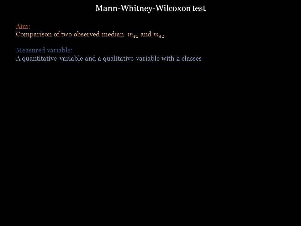
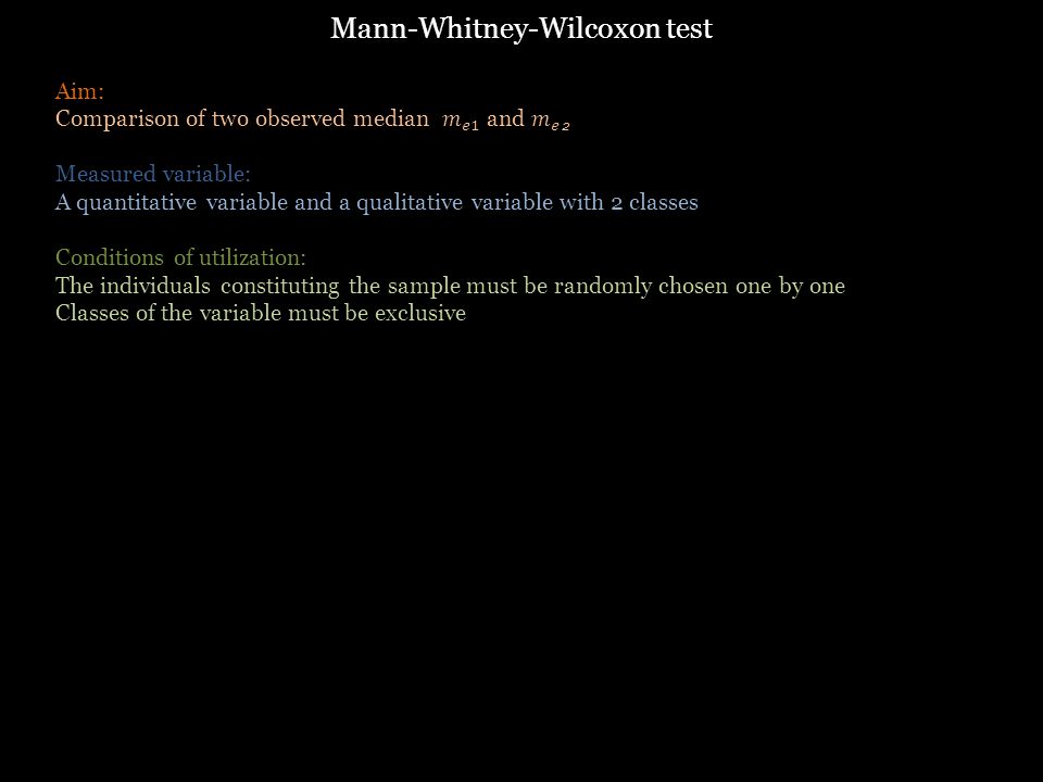
Mann-Whitney-Wilcoxon test

59
In R:W1calc-0.5*n1*(1+n1)
")
60
In details: Ceramics<-read.table("K:/Cours/Philippines/Statistics- 210/Data/Ceramics.txt",header=TRUE) obs1<-data.frame(Ceramics[which(Ceramics$Human.remains=="Yes" | Ceramics$Human.remains=="No"), c(4,14)]) obs1[, 2]<-factor(obs1[, 2]) obs2<-na.omit(obs1) Mann-Whitney-Wilcoxon test
![In details: Ceramics<-read.table( K:/Cours/Philippines/Statistics- 210/Data/Ceramics.txt ,header=TRUE) obs1<-data.frame(Ceramics[which(Ceramics$Human.remains== Yes | Ceramics$Human.remains== No ), c(4,14)]) obs1[, 2]<-factor(obs1[, 2]) obs2<-na.omit(obs1) Mann-Whitney-Wilcoxon test](http://images.slideplayer.com/11/3234051/slides/slide_60.jpg "In details: Ceramics<-read.table( K:/Cours/Philippines/Statistics- 210/Data/Ceramics.txt ,header=TRUE) obs1<-data.frame(Ceramics[which(Ceramics$Human.remains== Yes | Ceramics$Human.remains== No ), c(4,14)]) obs1[, 2]<-factor(obs1[, 2]) obs2<-na.omit(obs1) Mann-Whitney-Wilcoxon test")
61
In details: Ceramics<-read.table("K:/Cours/Philippines/Statistics- 210/Data/Ceramics.txt",header=TRUE) obs1<-data.frame(Ceramics[which(Ceramics$Human.remains=="Yes" | Ceramics$Human.remains=="No"), c(4,14)]) obs1[, 2]<-factor(obs1[, 2]) obs2<-na.omit(obs1) nc.max<-max(table(obs2[, 2])) nb.na<-nc.max- table(obs2[, 2]) tempo<-split(obs2[, 1], obs2[, 2]) for(i in 1:length(tempo)) {tempo[[i]]<-append(tempo[[i]],rep(NA,nb.na[i]))} Mann-Whitney-Wilcoxon test
![In details: Ceramics<-read.table( K:/Cours/Philippines/Statistics- 210/Data/Ceramics.txt ,header=TRUE) obs1<-data.frame(Ceramics[which(Ceramics$Human.remains== Yes | Ceramics$Human.remains== No ), c(4,14)]) obs1[, 2]<-factor(obs1[, 2]) obs2<-na.omit(obs1) nc.max<-max(table(obs2[, 2])) nb.na<-nc.max- table(obs2[, 2]) tempo<-split(obs2[, 1], obs2[, 2]) for(i in 1:length(tempo)) {tempo[[i]]<-append(tempo[[i]],rep(NA,nb.na[i]))} Mann-Whitney-Wilcoxon test](http://images.slideplayer.com/11/3234051/slides/slide_61.jpg "In details: Ceramics<-read.table( K:/Cours/Philippines/Statistics- 210/Data/Ceramics.txt ,header=TRUE) obs1<-data.frame(Ceramics[which(Ceramics$Human.remains== Yes | Ceramics$Human.remains== No ), c(4,14)]) obs1[, 2]<-factor(obs1[, 2]) obs2<-na.omit(obs1) nc.max<-max(table(obs2[, 2])) nb.na<-nc.max- table(obs2[, 2]) tempo<-split(obs2[, 1], obs2[, 2]) for(i in 1:length(tempo)) {tempo[[i]]<-append(tempo[[i]],rep(NA,nb.na[i]))} Mann-Whitney-Wilcoxon test")
62
In details: Ceramics<-read.table("K:/Cours/Philippines/Statistics- 210/Data/Ceramics.txt",header=TRUE) obs1<-data.frame(Ceramics[which(Ceramics$Human.remains=="Yes" | Ceramics$Human.remains=="No"), c(4,14)]) obs1[, 2]<-factor(obs1[, 2]) obs2<-na.omit(obs1) nc.max<-max(table(obs2[, 2])) nb.na<-nc.max- table(obs2[, 2]) tempo<-split(obs2[, 1], obs2[, 2]) for(i in 1:length(tempo)) {tempo[[i]]<-append(tempo[[i]],rep(NA,nb.na[i]))} obs3<-data.frame(tempo) xr<-sort(obs2[, 1]) ci<-obs2[, 2] cr<-ci[order(obs2[, 1])] r<-rank(xr,ties.method="average") obs4<-data.frame(r,xr,cr) names(obs4)<- c("rank", paste(names(obs2)[1], "by increasing order"), names(obs2)[2]) obs4 Mann-Whitney-Wilcoxon test
![In details: Ceramics<-read.table( K:/Cours/Philippines/Statistics- 210/Data/Ceramics.txt ,header=TRUE) obs1<-data.frame(Ceramics[which(Ceramics$Human.remains== Yes | Ceramics$Human.remains== No ), c(4,14)]) obs1[, 2]<-factor(obs1[, 2]) obs2<-na.omit(obs1) nc.max<-max(table(obs2[, 2])) nb.na<-nc.max- table(obs2[, 2]) tempo<-split(obs2[, 1], obs2[, 2]) for(i in 1:length(tempo)) {tempo[[i]]<-append(tempo[[i]],rep(NA,nb.na[i]))} obs3<-data.frame(tempo) xr<-sort(obs2[, 1]) ci<-obs2[, 2] cr<-ci[order(obs2[, 1])] r<-rank(xr,ties.method= average ) obs4<-data.frame(r,xr,cr) names(obs4)<- c( rank , paste(names(obs2)[1], by increasing order ), names(obs2)[2]) obs4 Mann-Whitney-Wilcoxon test](http://images.slideplayer.com/11/3234051/slides/slide_62.jpg "In details: Ceramics<-read.table( K:/Cours/Philippines/Statistics- 210/Data/Ceramics.txt ,header=TRUE) obs1<-data.frame(Ceramics[which(Ceramics$Human.remains== Yes | Ceramics$Human.remains== No ), c(4,14)]) obs1[, 2]<-factor(obs1[, 2]) obs2<-na.omit(obs1) nc.max<-max(table(obs2[, 2])) nb.na<-nc.max- table(obs2[, 2]) tempo<-split(obs2[, 1], obs2[, 2]) for(i in 1:length(tempo)) {tempo[[i]]<-append(tempo[[i]],rep(NA,nb.na[i]))} obs3<-data.frame(tempo) xr<-sort(obs2[, 1]) ci<-obs2[, 2] cr<-ci[order(obs2[, 1])] r<-rank(xr,ties.method= average ) obs4<-data.frame(r,xr,cr) names(obs4)<- c( rank , paste(names(obs2)[1], by increasing order ), names(obs2)[2]) obs4 Mann-Whitney-Wilcoxon test")
63
In details: n1<-sapply(split(obs2[, 1], obs2[, 2]), length)[1] n2<-sapply(split(obs2[, 1], obs2[, 2]), length)[2] m1<- sapply(split(obs2[, 1], obs2[, 2]), mean)[1] m2<- sapply(split(obs2[, 1], obs2[, 2]), mean)[2] s1<-sapply(split(obs2[, 1], obs2[, 2]), sd)[1] s2<-sapply(split(obs2[, 1], obs2[, 2]), sd)[2] me1<- sapply(split(obs2[, 1], obs2[, 2]), median)[1] me2<- sapply(split(obs2[, 1], obs2[, 2]), median)[2] min1<- sapply(split(obs2[, 1], obs2[, 2]), min)[1] min2<- sapply(split(obs2[, 1], obs2[, 2]), min)[2] max1<- sapply(split(obs2[, 1], obs2[, 2]), max)[1] max2<- sapply(split(obs2[, 1], obs2[, 2]), max)[2] Mann-Whitney-Wilcoxon test
![In details: n1<-sapply(split(obs2[, 1], obs2[, 2]), length)[1] n2<-sapply(split(obs2[, 1], obs2[, 2]), length)[2] m1<- sapply(split(obs2[, 1], obs2[, 2]), mean)[1] m2<- sapply(split(obs2[, 1], obs2[, 2]), mean)[2] s1<-sapply(split(obs2[, 1], obs2[, 2]), sd)[1] s2<-sapply(split(obs2[, 1], obs2[, 2]), sd)[2] me1<- sapply(split(obs2[, 1], obs2[, 2]), median)[1] me2<- sapply(split(obs2[, 1], obs2[, 2]), median)[2] min1<- sapply(split(obs2[, 1], obs2[, 2]), min)[1] min2<- sapply(split(obs2[, 1], obs2[, 2]), min)[2] max1<- sapply(split(obs2[, 1], obs2[, 2]), max)[1] max2<- sapply(split(obs2[, 1], obs2[, 2]), max)[2] Mann-Whitney-Wilcoxon test](http://images.slideplayer.com/11/3234051/slides/slide_63.jpg "In details: n1<-sapply(split(obs2[, 1], obs2[, 2]), length)[1] n2<-sapply(split(obs2[, 1], obs2[, 2]), length)[2] m1<- sapply(split(obs2[, 1], obs2[, 2]), mean)[1] m2<- sapply(split(obs2[, 1], obs2[, 2]), mean)[2] s1<-sapply(split(obs2[, 1], obs2[, 2]), sd)[1] s2<-sapply(split(obs2[, 1], obs2[, 2]), sd)[2] me1<- sapply(split(obs2[, 1], obs2[, 2]), median)[1] me2<- sapply(split(obs2[, 1], obs2[, 2]), median)[2] min1<- sapply(split(obs2[, 1], obs2[, 2]), min)[1] min2<- sapply(split(obs2[, 1], obs2[, 2]), min)[2] max1<- sapply(split(obs2[, 1], obs2[, 2]), max)[1] max2<- sapply(split(obs2[, 1], obs2[, 2]), max)[2] Mann-Whitney-Wilcoxon test")
64
In details: param <- data.frame(c(n1, n2), c(m1, m2), c(s1, s2), c(me1, me2), c(min1, min2), c(max1, max2)) names(param) <- c("Effective", "Mean", "Standard.deviation", "Median", "Minimum", "Maximum") row.names(levels(obs2[, 2])) param W1calc<-sum(subset(obs4[, 1], obs4[, 3]== names(obs3)[1])) U1calc<-W1calc-0.5*n1*(1+n1) U1calc min(pwilcox((U1calc-1), n1, n2, lower.tail=FALSE), pwilcox(U1calc, n1, n2))*2 Mann-Whitney-Wilcoxon test
![In details: param <- data.frame(c(n1, n2), c(m1, m2), c(s1, s2), c(me1, me2), c(min1, min2), c(max1, max2)) names(param) <- c( Effective , Mean , Standard.deviation , Median , Minimum , Maximum ) row.names(levels(obs2[, 2])) param W1calc<-sum(subset(obs4[, 1], obs4[, 3]== names(obs3)[1])) U1calc<-W1calc-0.5*n1*(1+n1) U1calc min(pwilcox((U1calc-1), n1, n2, lower.tail=FALSE), pwilcox(U1calc, n1, n2))*2 Mann-Whitney-Wilcoxon test](http://images.slideplayer.com/11/3234051/slides/slide_64.jpg "In details: param <- data.frame(c(n1, n2), c(m1, m2), c(s1, s2), c(me1, me2), c(min1, min2), c(max1, max2)) names(param) <- c( Effective , Mean , Standard.deviation , Median , Minimum , Maximum ) row.names(levels(obs2[, 2])) param W1calc<-sum(subset(obs4[, 1], obs4[, 3]== names(obs3)[1])) U1calc<-W1calc-0.5*n1*(1+n1) U1calc min(pwilcox((U1calc-1), n1, n2, lower.tail=FALSE), pwilcox(U1calc, n1, n2))*2 Mann-Whitney-Wilcoxon test")
65
In details: param <- data.frame(c(n1, n2), c(m1, m2), c(s1, s2), c(me1, me2), c(min1, min2), c(max1, max2)) names(param) <- c("Effective", "Mean", "Standard.deviation", "Median", "Minimum", "Maximum") row.names(levels(obs2[, 2])) param W1calc<-sum(subset(obs4[, 1], obs4[, 3]== names(obs3)[1])) U1calc<-W1calc-0.5*n1*(1+n1) U1calc min(pwilcox((U1calc-1), n1, n2, lower.tail=FALSE), pwilcox(U1calc, n1, n2))*2 ## In R wilcox.test(obs3[, 1], obs3[, 2]) Mann-Whitney-Wilcoxon test
![In details: param <- data.frame(c(n1, n2), c(m1, m2), c(s1, s2), c(me1, me2), c(min1, min2), c(max1, max2)) names(param) <- c( Effective , Mean , Standard.deviation , Median , Minimum , Maximum ) row.names(levels(obs2[, 2])) param W1calc<-sum(subset(obs4[, 1], obs4[, 3]== names(obs3)[1])) U1calc<-W1calc-0.5*n1*(1+n1) U1calc min(pwilcox((U1calc-1), n1, n2, lower.tail=FALSE), pwilcox(U1calc, n1, n2))*2 ## In R wilcox.test(obs3[, 1], obs3[, 2]) Mann-Whitney-Wilcoxon test](http://images.slideplayer.com/11/3234051/slides/slide_65.jpg "In details: param <- data.frame(c(n1, n2), c(m1, m2), c(s1, s2), c(me1, me2), c(min1, min2), c(max1, max2)) names(param) <- c( Effective , Mean , Standard.deviation , Median , Minimum , Maximum ) row.names(levels(obs2[, 2])) param W1calc<-sum(subset(obs4[, 1], obs4[, 3]== names(obs3)[1])) U1calc<-W1calc-0.5*n1*(1+n1) U1calc min(pwilcox((U1calc-1), n1, n2, lower.tail=FALSE), pwilcox(U1calc, n1, n2))*2 ## In R wilcox.test(obs3[, 1], obs3[, 2]) Mann-Whitney-Wilcoxon test")
66
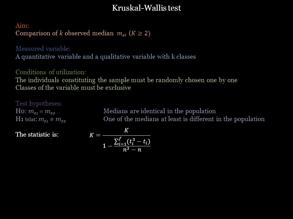
Kruskal-Wallis test

71
In details: Ceram<-read.table("K:/Cours/Philippines/Statistics- 210/Data/Ceramics.txt",header=TRUE) obs1<-Ceram[,c(7,10)] obs1[,2]<-factor(obs1[,2]) obs2<-na.omit(obs1) Kruskal-Wallis test
![In details: Ceram<-read.table( K:/Cours/Philippines/Statistics- 210/Data/Ceramics.txt ,header=TRUE) obs1<-Ceram[,c(7,10)] obs1[,2]<-factor(obs1[,2]) obs2<-na.omit(obs1) Kruskal-Wallis test](http://images.slideplayer.com/11/3234051/slides/slide_71.jpg "In details: Ceram<-read.table( K:/Cours/Philippines/Statistics- 210/Data/Ceramics.txt ,header=TRUE) obs1<-Ceram[,c(7,10)] obs1[,2]<-factor(obs1[,2]) obs2<-na.omit(obs1) Kruskal-Wallis test")
72
In details: Ceram<-read.table("K:/Cours/Philippines/Statistics- 210/Data/Ceramics.txt",header=TRUE) obs1<-Ceram[,c(7,10)] obs1[,2]<-factor(obs1[,2]) obs2<-na.omit(obs1) ri<-rank(obs2[,1],ties.method="average") obs3<-data.frame(obs2,ri) names(obs3)[3]<- "Rank" obs3 nc.max<-max(table(obs2[,2])) nb.na<-nc.max- table(obs2[,2]) tempo<-split(obs2[,1], obs2[,2]) for(i in 1:length(tempo)) {tempo[[i]]<-append(tempo[[i]],rep(NA,nb.na[i]))} obs4<-data.frame(tempo) Kruskal-Wallis test
![In details: Ceram<-read.table( K:/Cours/Philippines/Statistics- 210/Data/Ceramics.txt ,header=TRUE) obs1<-Ceram[,c(7,10)] obs1[,2]<-factor(obs1[,2]) obs2<-na.omit(obs1) ri<-rank(obs2[,1],ties.method= average ) obs3<-data.frame(obs2,ri) names(obs3)[3]<- Rank obs3 nc.max<-max(table(obs2[,2])) nb.na<-nc.max- table(obs2[,2]) tempo<-split(obs2[,1], obs2[,2]) for(i in 1:length(tempo)) {tempo[[i]]<-append(tempo[[i]],rep(NA,nb.na[i]))} obs4<-data.frame(tempo) Kruskal-Wallis test](http://images.slideplayer.com/11/3234051/slides/slide_72.jpg "In details: Ceram<-read.table( K:/Cours/Philippines/Statistics- 210/Data/Ceramics.txt ,header=TRUE) obs1<-Ceram[,c(7,10)] obs1[,2]<-factor(obs1[,2]) obs2<-na.omit(obs1) ri<-rank(obs2[,1],ties.method= average ) obs3<-data.frame(obs2,ri) names(obs3)[3]<- Rank obs3 nc.max<-max(table(obs2[,2])) nb.na<-nc.max- table(obs2[,2]) tempo<-split(obs2[,1], obs2[,2]) for(i in 1:length(tempo)) {tempo[[i]]<-append(tempo[[i]],rep(NA,nb.na[i]))} obs4<-data.frame(tempo) Kruskal-Wallis test")
73
In details: nc<-sapply(split(obs2[, 1], obs2[, 2]), length) me.c<-sapply(split(obs2[,1], obs2[,2]), median) min.c<- sapply(split(obs2[,1], obs2[,2]), min) max.c<- sapply(split(obs2[,1], obs2[,2]), max) mc<-sapply(split(obs2[, 1], obs2[, 2]), mean) sc<-sapply(split(obs2[, 1], obs2[, 2]), sd) param <- data.frame(nc, me.c, min.c, max.c, mc, sc) names(param) <- c("Effective", "Median", "Minimum", "Maximum", "Mean", "Standard.deviation") row.names(levels(obs2[, 2])) param Kruskal-Wallis test
![In details: nc<-sapply(split(obs2[, 1], obs2[, 2]), length) me.c<-sapply(split(obs2[,1], obs2[,2]), median) min.c<- sapply(split(obs2[,1], obs2[,2]), min) max.c<- sapply(split(obs2[,1], obs2[,2]), max) mc<-sapply(split(obs2[, 1], obs2[, 2]), mean) sc<-sapply(split(obs2[, 1], obs2[, 2]), sd) param <- data.frame(nc, me.c, min.c, max.c, mc, sc) names(param) <- c( Effective , Median , Minimum , Maximum , Mean , Standard.deviation ) row.names(levels(obs2[, 2])) param Kruskal-Wallis test](http://images.slideplayer.com/11/3234051/slides/slide_73.jpg "In details: nc<-sapply(split(obs2[, 1], obs2[, 2]), length) me.c<-sapply(split(obs2[,1], obs2[,2]), median) min.c<- sapply(split(obs2[,1], obs2[,2]), min) max.c<- sapply(split(obs2[,1], obs2[,2]), max) mc<-sapply(split(obs2[, 1], obs2[, 2]), mean) sc<-sapply(split(obs2[, 1], obs2[, 2]), sd) param <- data.frame(nc, me.c, min.c, max.c, mc, sc) names(param) <- c( Effective , Median , Minimum , Maximum , Mean , Standard.deviation ) row.names(levels(obs2[, 2])) param Kruskal-Wallis test")
74
In details: n<-length(obs3$Rank) Rc<-tapply(obs3$Rank, obs3[, 2], "sum") K.calc<-12*sum(Rc^2/nc)/(n*(n+1))-3*(n+1) K.calc ti<-table(obs3[,1]) Kcorr<-K.calc/(1-sum(ti^3-ti)/(n^3-n)) Kcorr k<-length(nc) pchisq(Kcorr, k-1, lower.tail=FALSE) k<-length(nc) n<-sum(nc) vecteur.ini<-NULL for(i in 1:k){vecteur.ini<-c(vecteur.ini, rep(LETTERS[i], nc[i]))} rank<-1:n ## Test in R kruskal.test(obs1[,1], obs1[,2]) Kruskal-Wallis test
![In details: n<-length(obs3$Rank) Rc<-tapply(obs3$Rank, obs3[, 2], sum ) K.calc<-12*sum(Rc^2/nc)/(n*(n+1))-3*(n+1) K.calc ti<-table(obs3[,1]) Kcorr<-K.calc/(1-sum(ti^3-ti)/(n^3-n)) Kcorr k<-length(nc) pchisq(Kcorr, k-1, lower.tail=FALSE) k<-length(nc) n<-sum(nc) vecteur.ini<-NULL for(i in 1:k){vecteur.ini<-c(vecteur.ini, rep(LETTERS[i], nc[i]))} rank<-1:n ## Test in R kruskal.test(obs1[,1], obs1[,2]) Kruskal-Wallis test](http://images.slideplayer.com/11/3234051/slides/slide_74.jpg "In details: n<-length(obs3$Rank) Rc<-tapply(obs3$Rank, obs3[, 2], sum ) K.calc<-12*sum(Rc^2/nc)/(n*(n+1))-3*(n+1) K.calc ti<-table(obs3[,1]) Kcorr<-K.calc/(1-sum(ti^3-ti)/(n^3-n)) Kcorr k<-length(nc) pchisq(Kcorr, k-1, lower.tail=FALSE) k<-length(nc) n<-sum(nc) vecteur.ini<-NULL for(i in 1:k){vecteur.ini<-c(vecteur.ini, rep(LETTERS[i], nc[i]))} rank<-1:n ## Test in R kruskal.test(obs1[,1], obs1[,2]) Kruskal-Wallis test")
75
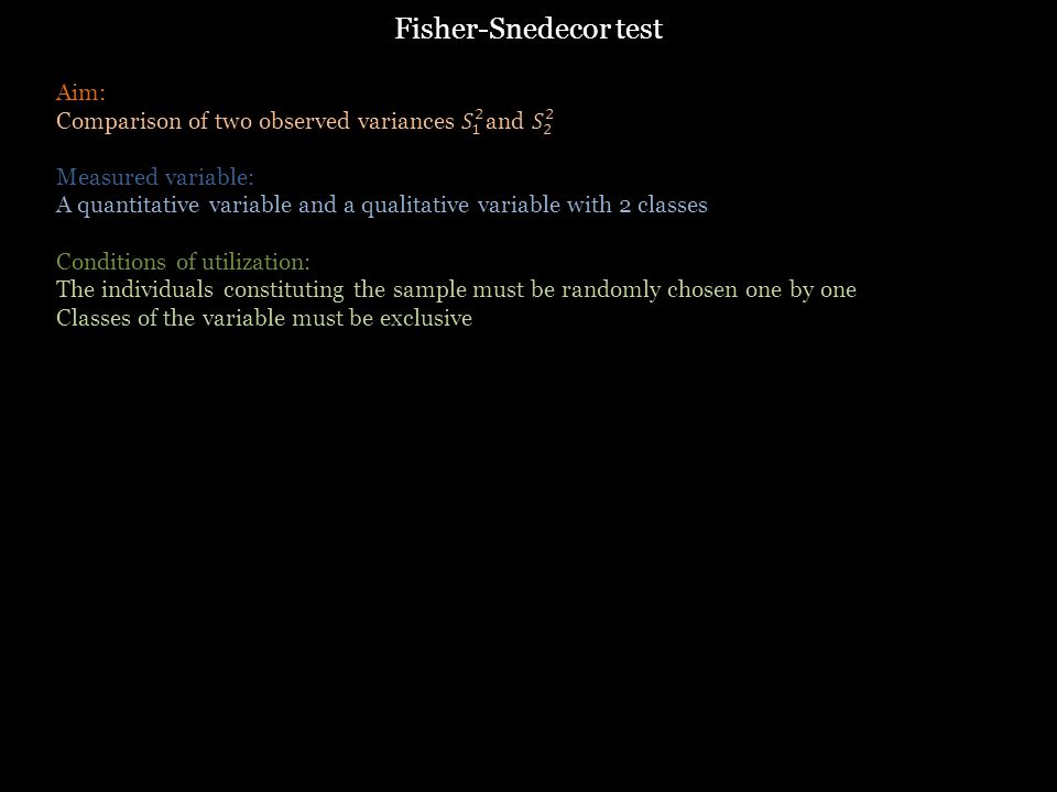
Fisher-Snedecor test

80
In details: n<-length(obs3$Rank) Rc<-tapply(obs3$Rank, obs3[, 2], "sum") K.calc<-12*sum(Rc^2/nc)/(n*(n+1))-3*(n+1) K.calc ti<-table(obs3[,1]) Kcorr<-K.calc/(1-sum(ti^3-ti)/(n^3-n)) Kcorr k<-length(nc) pchisq(Kcorr, k-1, lower.tail=FALSE) k<-length(nc) n<-sum(nc) vecteur.ini<-NULL for(i in 1:k){vecteur.ini<-c(vecteur.ini, rep(LETTERS[i], nc[i]))} rank<-1:n ## Test in R kruskal.test(obs1[,1], obs1[,2]) Fisher-Snedecor test
![In details: n<-length(obs3$Rank) Rc<-tapply(obs3$Rank, obs3[, 2], sum ) K.calc<-12*sum(Rc^2/nc)/(n*(n+1))-3*(n+1) K.calc ti<-table(obs3[,1]) Kcorr<-K.calc/(1-sum(ti^3-ti)/(n^3-n)) Kcorr k<-length(nc) pchisq(Kcorr, k-1, lower.tail=FALSE) k<-length(nc) n<-sum(nc) vecteur.ini<-NULL for(i in 1:k){vecteur.ini<-c(vecteur.ini, rep(LETTERS[i], nc[i]))} rank<-1:n ## Test in R kruskal.test(obs1[,1], obs1[,2]) Fisher-Snedecor test](http://images.slideplayer.com/11/3234051/slides/slide_80.jpg "In details: n<-length(obs3$Rank) Rc<-tapply(obs3$Rank, obs3[, 2], sum ) K.calc<-12*sum(Rc^2/nc)/(n*(n+1))-3*(n+1) K.calc ti<-table(obs3[,1]) Kcorr<-K.calc/(1-sum(ti^3-ti)/(n^3-n)) Kcorr k<-length(nc) pchisq(Kcorr, k-1, lower.tail=FALSE) k<-length(nc) n<-sum(nc) vecteur.ini<-NULL for(i in 1:k){vecteur.ini<-c(vecteur.ini, rep(LETTERS[i], nc[i]))} rank<-1:n ## Test in R kruskal.test(obs1[,1], obs1[,2]) Fisher-Snedecor test")
81
In details: Ceram<-read.table("K:/Cours/Philippines/Statistics- 210/Data/Ceramics.txt",header=TRUE) obs1<-data.frame(Ceram[which(Ceram$Base=="Round" | Ceram$Base=="Flat"), c(6,13)]) obs1[,2]<-factor(obs1[,2]) obs2<-na.omit(obs1) Fisher-Snedecor test
![In details: Ceram<-read.table( K:/Cours/Philippines/Statistics- 210/Data/Ceramics.txt ,header=TRUE) obs1<-data.frame(Ceram[which(Ceram$Base== Round | Ceram$Base== Flat ), c(6,13)]) obs1[,2]<-factor(obs1[,2]) obs2<-na.omit(obs1) Fisher-Snedecor test](http://images.slideplayer.com/11/3234051/slides/slide_81.jpg "In details: Ceram<-read.table( K:/Cours/Philippines/Statistics- 210/Data/Ceramics.txt ,header=TRUE) obs1<-data.frame(Ceram[which(Ceram$Base== Round | Ceram$Base== Flat ), c(6,13)]) obs1[,2]<-factor(obs1[,2]) obs2<-na.omit(obs1) Fisher-Snedecor test")
82
In details: Ceram<-read.table("K:/Cours/Philippines/Statistics- 210/Data/Ceramics.txt",header=TRUE) obs1<-data.frame(Ceram[which(Ceram$Base=="Round" | Ceram$Base=="Flat"), c(6,13)]) obs1[,2]<-factor(obs1[,2]) obs2<-na.omit(obs1) nc.max<-max(table(obs2[,2])) nb.na<-nc.max- table(obs2[,2]) tempo<-split(obs2[,1], obs2[,2]) for(i in 1:length(tempo)) {tempo[[i]]<-append(tempo[[i]],rep(NA,nb.na[i]))} obs3<-data.frame(tempo) obs3 Fisher-Snedecor test
![In details: Ceram<-read.table( K:/Cours/Philippines/Statistics- 210/Data/Ceramics.txt ,header=TRUE) obs1<-data.frame(Ceram[which(Ceram$Base== Round | Ceram$Base== Flat ), c(6,13)]) obs1[,2]<-factor(obs1[,2]) obs2<-na.omit(obs1) nc.max<-max(table(obs2[,2])) nb.na<-nc.max- table(obs2[,2]) tempo<-split(obs2[,1], obs2[,2]) for(i in 1:length(tempo)) {tempo[[i]]<-append(tempo[[i]],rep(NA,nb.na[i]))} obs3<-data.frame(tempo) obs3 Fisher-Snedecor test](http://images.slideplayer.com/11/3234051/slides/slide_82.jpg "In details: Ceram<-read.table( K:/Cours/Philippines/Statistics- 210/Data/Ceramics.txt ,header=TRUE) obs1<-data.frame(Ceram[which(Ceram$Base== Round | Ceram$Base== Flat ), c(6,13)]) obs1[,2]<-factor(obs1[,2]) obs2<-na.omit(obs1) nc.max<-max(table(obs2[,2])) nb.na<-nc.max- table(obs2[,2]) tempo<-split(obs2[,1], obs2[,2]) for(i in 1:length(tempo)) {tempo[[i]]<-append(tempo[[i]],rep(NA,nb.na[i]))} obs3<-data.frame(tempo) obs3 Fisher-Snedecor test")
83
In details: Ceram<-read.table("K:/Cours/Philippines/Statistics- 210/Data/Ceramics.txt",header=TRUE) obs1<-data.frame(Ceram[which(Ceram$Base=="Round" | Ceram$Base=="Flat"), c(6,13)]) obs1[,2]<-factor(obs1[,2]) obs2<-na.omit(obs1) nc.max<-max(table(obs2[,2])) nb.na<-nc.max- table(obs2[,2]) tempo<-split(obs2[,1], obs2[,2]) for(i in 1:length(tempo)) {tempo[[i]]<-append(tempo[[i]],rep(NA,nb.na[i]))} obs3<-data.frame(tempo) obs3 mc<-sapply(split(obs2[,1], obs2[,2]),mean) obs4<-obs2 obs4[which(obs2[, 2] == levels(obs2[, 2])[1]), 1] <- obs4[which(obs2[, 2] == levels(obs2[, 2])[1]), 1] - mc[1] obs4[which(obs2[, 2] == levels(obs2[, 2])[2]), 1] <- obs4[which(obs2[, 2] == levels(obs2[, 2])[2]), 1] - mc[2] Fisher-Snedecor test
![In details: Ceram<-read.table( K:/Cours/Philippines/Statistics- 210/Data/Ceramics.txt ,header=TRUE) obs1<-data.frame(Ceram[which(Ceram$Base== Round | Ceram$Base== Flat ), c(6,13)]) obs1[,2]<-factor(obs1[,2]) obs2<-na.omit(obs1) nc.max<-max(table(obs2[,2])) nb.na<-nc.max- table(obs2[,2]) tempo<-split(obs2[,1], obs2[,2]) for(i in 1:length(tempo)) {tempo[[i]]<-append(tempo[[i]],rep(NA,nb.na[i]))} obs3<-data.frame(tempo) obs3 mc<-sapply(split(obs2[,1], obs2[,2]),mean) obs4<-obs2 obs4[which(obs2[, 2] == levels(obs2[, 2])[1]), 1] <- obs4[which(obs2[, 2] == levels(obs2[, 2])[1]), 1] - mc[1] obs4[which(obs2[, 2] == levels(obs2[, 2])[2]), 1] <- obs4[which(obs2[, 2] == levels(obs2[, 2])[2]), 1] - mc[2] Fisher-Snedecor test](http://images.slideplayer.com/11/3234051/slides/slide_83.jpg "In details: Ceram<-read.table( K:/Cours/Philippines/Statistics- 210/Data/Ceramics.txt ,header=TRUE) obs1<-data.frame(Ceram[which(Ceram$Base== Round | Ceram$Base== Flat ), c(6,13)]) obs1[,2]<-factor(obs1[,2]) obs2<-na.omit(obs1) nc.max<-max(table(obs2[,2])) nb.na<-nc.max- table(obs2[,2]) tempo<-split(obs2[,1], obs2[,2]) for(i in 1:length(tempo)) {tempo[[i]]<-append(tempo[[i]],rep(NA,nb.na[i]))} obs3<-data.frame(tempo) obs3 mc<-sapply(split(obs2[,1], obs2[,2]),mean) obs4<-obs2 obs4[which(obs2[, 2] == levels(obs2[, 2])[1]), 1] <- obs4[which(obs2[, 2] == levels(obs2[, 2])[1]), 1] - mc[1] obs4[which(obs2[, 2] == levels(obs2[, 2])[2]), 1] <- obs4[which(obs2[, 2] == levels(obs2[, 2])[2]), 1] - mc[2] Fisher-Snedecor test")
84
In details: n1<-sapply(split(obs2[, 1], obs2[, 2]), length)[1] n2<-sapply(split(obs2[, 1], obs2[, 2]), length)[2] s2.1<-sapply(split(obs2[, 1], obs2[, 2]), var)[1] s2.2<-sapply(split(obs2[, 1], obs2[, 2]), var)[2] m1<- sapply(split(obs2[, 1], obs2[, 2]), mean)[1] m2<- sapply(split(obs2[, 1], obs2[, 2]), mean)[2] param <- data.frame(c(n1, n2), c(s2.1, s2.2), c(s2.1^0.5, s2.2^0.5), c(m1, m2)) names(param) <- c("Effective", "Variance", « Standard.deviation", "Mean") row.names(levels(obs2[, 2])) param Fisher-Snedecor test
![In details: n1<-sapply(split(obs2[, 1], obs2[, 2]), length)[1] n2<-sapply(split(obs2[, 1], obs2[, 2]), length)[2] s2.1<-sapply(split(obs2[, 1], obs2[, 2]), var)[1] s2.2<-sapply(split(obs2[, 1], obs2[, 2]), var)[2] m1<- sapply(split(obs2[, 1], obs2[, 2]), mean)[1] m2<- sapply(split(obs2[, 1], obs2[, 2]), mean)[2] param <- data.frame(c(n1, n2), c(s2.1, s2.2), c(s2.1^0.5, s2.2^0.5), c(m1, m2)) names(param) <- c( Effective , Variance , « Standard.deviation , Mean ) row.names(levels(obs2[, 2])) param Fisher-Snedecor test](http://images.slideplayer.com/11/3234051/slides/slide_84.jpg "In details: n1<-sapply(split(obs2[, 1], obs2[, 2]), length)[1] n2<-sapply(split(obs2[, 1], obs2[, 2]), length)[2] s2.1<-sapply(split(obs2[, 1], obs2[, 2]), var)[1] s2.2<-sapply(split(obs2[, 1], obs2[, 2]), var)[2] m1<- sapply(split(obs2[, 1], obs2[, 2]), mean)[1] m2<- sapply(split(obs2[, 1], obs2[, 2]), mean)[2] param <- data.frame(c(n1, n2), c(s2.1, s2.2), c(s2.1^0.5, s2.2^0.5), c(m1, m2)) names(param) <- c( Effective , Variance , « Standard.deviation , Mean ) row.names(levels(obs2[, 2])) param Fisher-Snedecor test")
85
In details: n1<-sapply(split(obs2[, 1], obs2[, 2]), length)[1] n2<-sapply(split(obs2[, 1], obs2[, 2]), length)[2] s2.1<-sapply(split(obs2[, 1], obs2[, 2]), var)[1] s2.2<-sapply(split(obs2[, 1], obs2[, 2]), var)[2] m1<- sapply(split(obs2[, 1], obs2[, 2]), mean)[1] m2<- sapply(split(obs2[, 1], obs2[, 2]), mean)[2] param <- data.frame(c(n1, n2), c(s2.1, s2.2), c(s2.1^0.5, s2.2^0.5), c(m1, m2)) names(param) <- c("Effective", "Variance", « Standard.deviation", "Mean") row.names(levels(obs2[, 2])) param F.calc<-s2.1/s2.2 F.calc nu.1<-n1-1 nu.2<-n2-1 min(pf(F.calc, nu.1, nu.2, lower.tail=FALSE), pf(F.calc, nu.1, nu.2))*2 F.calc/qf(0.025, nu.1, nu.2, lower.tail=FALSE) F.calc/qf(0.025, nu.1, nu.2) Fisher-Snedecor test
![In details: n1<-sapply(split(obs2[, 1], obs2[, 2]), length)[1] n2<-sapply(split(obs2[, 1], obs2[, 2]), length)[2] s2.1<-sapply(split(obs2[, 1], obs2[, 2]), var)[1] s2.2<-sapply(split(obs2[, 1], obs2[, 2]), var)[2] m1<- sapply(split(obs2[, 1], obs2[, 2]), mean)[1] m2<- sapply(split(obs2[, 1], obs2[, 2]), mean)[2] param <- data.frame(c(n1, n2), c(s2.1, s2.2), c(s2.1^0.5, s2.2^0.5), c(m1, m2)) names(param) <- c( Effective , Variance , « Standard.deviation , Mean ) row.names(levels(obs2[, 2])) param F.calc<-s2.1/s2.2 F.calc nu.1<-n1-1 nu.2<-n2-1 min(pf(F.calc, nu.1, nu.2, lower.tail=FALSE), pf(F.calc, nu.1, nu.2))*2 F.calc/qf(0.025, nu.1, nu.2, lower.tail=FALSE) F.calc/qf(0.025, nu.1, nu.2) Fisher-Snedecor test](http://images.slideplayer.com/11/3234051/slides/slide_85.jpg "In details: n1<-sapply(split(obs2[, 1], obs2[, 2]), length)[1] n2<-sapply(split(obs2[, 1], obs2[, 2]), length)[2] s2.1<-sapply(split(obs2[, 1], obs2[, 2]), var)[1] s2.2<-sapply(split(obs2[, 1], obs2[, 2]), var)[2] m1<- sapply(split(obs2[, 1], obs2[, 2]), mean)[1] m2<- sapply(split(obs2[, 1], obs2[, 2]), mean)[2] param <- data.frame(c(n1, n2), c(s2.1, s2.2), c(s2.1^0.5, s2.2^0.5), c(m1, m2)) names(param) <- c( Effective , Variance , « Standard.deviation , Mean ) row.names(levels(obs2[, 2])) param F.calc<-s2.1/s2.2 F.calc nu.1<-n1-1 nu.2<-n2-1 min(pf(F.calc, nu.1, nu.2, lower.tail=FALSE), pf(F.calc, nu.1, nu.2))*2 F.calc/qf(0.025, nu.1, nu.2, lower.tail=FALSE) F.calc/qf(0.025, nu.1, nu.2) Fisher-Snedecor test")
86
In details: n1<-sapply(split(obs2[, 1], obs2[, 2]), length)[1] n2<-sapply(split(obs2[, 1], obs2[, 2]), length)[2] s2.1<-sapply(split(obs2[, 1], obs2[, 2]), var)[1] s2.2<-sapply(split(obs2[, 1], obs2[, 2]), var)[2] m1<- sapply(split(obs2[, 1], obs2[, 2]), mean)[1] m2<- sapply(split(obs2[, 1], obs2[, 2]), mean)[2] param <- data.frame(c(n1, n2), c(s2.1, s2.2), c(s2.1^0.5, s2.2^0.5), c(m1, m2)) names(param) <- c("Effective", "Variance", « Standard.deviation", "Mean") row.names(levels(obs2[, 2])) param F.calc<-s2.1/s2.2 F.calc nu.1<-n1-1 nu.2<-n2-1 min(pf(F.calc, nu.1, nu.2, lower.tail=FALSE), pf(F.calc, nu.1, nu.2))*2 F.calc/qf(0.025, nu.1, nu.2, lower.tail=FALSE) F.calc/qf(0.025, nu.1, nu.2) ## In R var.test(obs3[, 1], obs3[, 2]) Fisher-Snedecor test
![In details: n1<-sapply(split(obs2[, 1], obs2[, 2]), length)[1] n2<-sapply(split(obs2[, 1], obs2[, 2]), length)[2] s2.1<-sapply(split(obs2[, 1], obs2[, 2]), var)[1] s2.2<-sapply(split(obs2[, 1], obs2[, 2]), var)[2] m1<- sapply(split(obs2[, 1], obs2[, 2]), mean)[1] m2<- sapply(split(obs2[, 1], obs2[, 2]), mean)[2] param <- data.frame(c(n1, n2), c(s2.1, s2.2), c(s2.1^0.5, s2.2^0.5), c(m1, m2)) names(param) <- c( Effective , Variance , « Standard.deviation , Mean ) row.names(levels(obs2[, 2])) param F.calc<-s2.1/s2.2 F.calc nu.1<-n1-1 nu.2<-n2-1 min(pf(F.calc, nu.1, nu.2, lower.tail=FALSE), pf(F.calc, nu.1, nu.2))*2 F.calc/qf(0.025, nu.1, nu.2, lower.tail=FALSE) F.calc/qf(0.025, nu.1, nu.2) ## In R var.test(obs3[, 1], obs3[, 2]) Fisher-Snedecor test](http://images.slideplayer.com/11/3234051/slides/slide_86.jpg "In details: n1<-sapply(split(obs2[, 1], obs2[, 2]), length)[1] n2<-sapply(split(obs2[, 1], obs2[, 2]), length)[2] s2.1<-sapply(split(obs2[, 1], obs2[, 2]), var)[1] s2.2<-sapply(split(obs2[, 1], obs2[, 2]), var)[2] m1<- sapply(split(obs2[, 1], obs2[, 2]), mean)[1] m2<- sapply(split(obs2[, 1], obs2[, 2]), mean)[2] param <- data.frame(c(n1, n2), c(s2.1, s2.2), c(s2.1^0.5, s2.2^0.5), c(m1, m2)) names(param) <- c( Effective , Variance , « Standard.deviation , Mean ) row.names(levels(obs2[, 2])) param F.calc<-s2.1/s2.2 F.calc nu.1<-n1-1 nu.2<-n2-1 min(pf(F.calc, nu.1, nu.2, lower.tail=FALSE), pf(F.calc, nu.1, nu.2))*2 F.calc/qf(0.025, nu.1, nu.2, lower.tail=FALSE) F.calc/qf(0.025, nu.1, nu.2) ## In R var.test(obs3[, 1], obs3[, 2]) Fisher-Snedecor test")
87
Spearman correlation test In R:n*(n^2-1)*(1-rho.xy)/6
*(1-rho.xy)/6")
88
In details: Ceram<-read.table("K:/Cours/Philippines/Statistics- 210/Data/Ceramics.txt",header=TRUE) obs1<-data.frame(Ceram[which(Ceram$Human.remains=="Yes"), c(2,4)]) obs2<-na.omit(obs1) Spearman correlation test
![In details: Ceram<-read.table( K:/Cours/Philippines/Statistics- 210/Data/Ceramics.txt ,header=TRUE) obs1<-data.frame(Ceram[which(Ceram$Human.remains== Yes ), c(2,4)]) obs2<-na.omit(obs1) Spearman correlation test](http://images.slideplayer.com/11/3234051/slides/slide_88.jpg "In details: Ceram<-read.table( K:/Cours/Philippines/Statistics- 210/Data/Ceramics.txt ,header=TRUE) obs1<-data.frame(Ceram[which(Ceram$Human.remains== Yes ), c(2,4)]) obs2<-na.omit(obs1) Spearman correlation test")
89
In details: Ceram<-read.table("K:/Cours/Philippines/Statistics- 210/Data/Ceramics.txt",header=TRUE) obs1<-data.frame(Ceram[which(Ceram$Human.remains=="Yes"), c(2,4)]) obs2<-na.omit(obs1) rxi<-rank(obs2[,1],ties.method = "average") ryi<-rank(obs2[,2],ties.method = "average") obs3<-data.frame(rxi,ryi) names(obs3)<-c(paste("rank of", names(obs2)[1]), paste("rank of", names(obs2)[2])) obs3 Spearman correlation test
![In details: Ceram<-read.table( K:/Cours/Philippines/Statistics- 210/Data/Ceramics.txt ,header=TRUE) obs1<-data.frame(Ceram[which(Ceram$Human.remains== Yes ), c(2,4)]) obs2<-na.omit(obs1) rxi<-rank(obs2[,1],ties.method = average ) ryi<-rank(obs2[,2],ties.method = average ) obs3<-data.frame(rxi,ryi) names(obs3)<-c(paste( rank of , names(obs2)[1]), paste( rank of , names(obs2)[2])) obs3 Spearman correlation test](http://images.slideplayer.com/11/3234051/slides/slide_89.jpg "In details: Ceram<-read.table( K:/Cours/Philippines/Statistics- 210/Data/Ceramics.txt ,header=TRUE) obs1<-data.frame(Ceram[which(Ceram$Human.remains== Yes ), c(2,4)]) obs2<-na.omit(obs1) rxi<-rank(obs2[,1],ties.method = average ) ryi<-rank(obs2[,2],ties.method = average ) obs3<-data.frame(rxi,ryi) names(obs3)<-c(paste( rank of , names(obs2)[1]), paste( rank of , names(obs2)[2])) obs3 Spearman correlation test")
90
In details: Ceram<-read.table("K:/Cours/Philippines/Statistics- 210/Data/Ceramics.txt",header=TRUE) obs1<-data.frame(Ceram[which(Ceram$Human.remains=="Yes"), c(2,4)]) obs2<-na.omit(obs1) rxi<-rank(obs2[,1],ties.method = "average") ryi<-rank(obs2[,2],ties.method = "average") obs3<-data.frame(rxi,ryi) names(obs3)<-c(paste("rank of", names(obs2)[1]), paste("rank of", names(obs2)[2])) obs3 n<-length(obs2[, 1]) n rho.xy<-(sum(rxi*ryi) - n*((n+1)/2)^2) / ((sum(rxi^2) - n*((n+1)/2)^2)^0.5 * (sum(ryi^2) -n*((n+1)/2)^2)^0.5) rho.xy cor(rank(obs2[,1]), rank(obs2[,2])) Scalc<-n*(n^2-1)*(1-rho.xy)/6 Scalc sum((ryi-rxi)^2) Spearman correlation test
![In details: Ceram<-read.table( K:/Cours/Philippines/Statistics- 210/Data/Ceramics.txt ,header=TRUE) obs1<-data.frame(Ceram[which(Ceram$Human.remains== Yes ), c(2,4)]) obs2<-na.omit(obs1) rxi<-rank(obs2[,1],ties.method = average ) ryi<-rank(obs2[,2],ties.method = average ) obs3<-data.frame(rxi,ryi) names(obs3)<-c(paste( rank of , names(obs2)[1]), paste( rank of , names(obs2)[2])) obs3 n<-length(obs2[, 1]) n rho.xy<-(sum(rxi*ryi) - n*((n+1)/2)^2) / ((sum(rxi^2) - n*((n+1)/2)^2)^0.5 * (sum(ryi^2) -n*((n+1)/2)^2)^0.5) rho.xy cor(rank(obs2[,1]), rank(obs2[,2])) Scalc<-n*(n^2-1)*(1-rho.xy)/6 Scalc sum((ryi-rxi)^2) Spearman correlation test](http://images.slideplayer.com/11/3234051/slides/slide_90.jpg "In details: Ceram<-read.table( K:/Cours/Philippines/Statistics- 210/Data/Ceramics.txt ,header=TRUE) obs1<-data.frame(Ceram[which(Ceram$Human.remains== Yes ), c(2,4)]) obs2<-na.omit(obs1) rxi<-rank(obs2[,1],ties.method = average ) ryi<-rank(obs2[,2],ties.method = average ) obs3<-data.frame(rxi,ryi) names(obs3)<-c(paste( rank of , names(obs2)[1]), paste( rank of , names(obs2)[2])) obs3 n<-length(obs2[, 1]) n rho.xy<-(sum(rxi*ryi) - n*((n+1)/2)^2) / ((sum(rxi^2) - n*((n+1)/2)^2)^0.5 * (sum(ryi^2) -n*((n+1)/2)^2)^0.5) rho.xy cor(rank(obs2[,1]), rank(obs2[,2])) Scalc<-n*(n^2-1)*(1-rho.xy)/6 Scalc sum((ryi-rxi)^2) Spearman correlation test")
91
In details: ## In R cor.test(obs1[,1], obs1[,2], method="spearman") Spearman correlation test
![In details: ## In R cor.test(obs1[,1], obs1[,2], method= spearman ) Spearman correlation test](http://images.slideplayer.com/11/3234051/slides/slide_91.jpg "In details: ## In R cor.test(obs1[,1], obs1[,2], method= spearman ) Spearman correlation test")
Similar presentations


 DISTRIBUTION>")


 1.>")
