2. Topic Outline

3. ? Black-Box Optimization Optimization Algorithm: only allowed to evaluate f (direct search) decision vector x objective vector f(x) objective function (e.g. simulation model)

4. So what is the general problem? The Multiobjective optimization problem (MOP) can be defined as the problem of finding [Osyczka 1985] a vector of decision variables which satisfies constraints and optimizes a vector function show elements represent the objective functions. Hence, the term “optimize” means finding such a solution which would give the values of all objective functions acceptable to the designer.

5. What does optimum mean here? Having several objective functions implies that we are trying to find a good compromise rather than a single optimal solution. Francis Ysidro Edgeworth first proposed a meaning for “optimum” in 1881 which was generalized in 1896 by Vilfredo Pareto

6. Mapping from decision space to objective space assuming maximization:

7. dominance

8. Pareto Optimal Fronts

9. Issues in EMO y2y2 y1y1 Diversity Convergence How to maintain a diverse Pareto set approximation?  density estimation How to prevent nondominated solutions from being lost?  environmental selection How to guide the population towards the Pareto set?  fitness assignment

10. General Diversity Preservation Various techniques are available for maintaining diversity in a MOEA like: Weight Vector Approach the Fitness Sharing/Niching Approach Crowding/Clustering Restricted Mating Relaxed Dominance

11. A graphical illustration of fitness sharing

12. density estimation Kernel approach: The density estimator is based on the sum of F values, where F is a function of the distance (vector) measured either in genotypic or in phenotypic space (e.g., MOGA and the NPGA). Nearest neighbor approach: The density estimator is based on the volume of the hyper-rectangle defined by the nearest neighbors (e.g., the NSGA-II and SPEA2). Histogram approach : The density estimator is based on the number of solutions that lie within the same hyper-box (e.g., PAES and PESA).

14. Classifying EMOO approaches (Evolutionary Multi-Objective Optimization) First Generation Techniques Non-Pareto approaches Pareto approaches Second Generation Techniques PAES SPEA NSGA-II MOMGA micro-GA

15. Non-Pareto Techniques These are methods that do not use information about Pareto fronts explicitly. Incapable of producing certain portions of the Pareto front. Efficient and easy to implement, but appropriate to handle only a few objectives.

16. Aggregate Objective Model (weighted sum method) Aggregated fitness functions are basically just a weighted sum of the objective functions. This is what we did in Landscape smoothing. The weighted sum creates a single objective function from the multi-objective fitness function. Determining the weights to use in this sum is non trivial and is almost always problem dependent.

17. Aggregate Function The weighted sum is basically in the following form. where represents the weights often we assume

18. Weighted Sum Method Construct a weighted sum of Objectives and optimize User supplies weight vector w

19. Disadvantage Need to know w Non-uniformity in Pareto- Optimal solutions Inability to find some Pareto- optimal solution

20. Vector Evaluated Genetic Algorithm (VEGA) This work was performed by J. D. Schaffer in 1985 and can be found in paper Schaffer, J.D., Multiple objective optimization with vector evaluated genetic algorithms. In this method appropriate fractions of the next generation, or subpopulations, were selected from the whole of the old generation according to each of the objectives, separately. Crossover and mutation were applied as usual after combining the sub-populations

21. Schematic of VEGA selection step 1 step 2 step 3 select n subgroups using each objective in turn shuffleapply genetic operators n 1 2 …... geneperformance n 12... popSize 1 …...... gen ( t )parentsgen ( t +1) popSize 1 …...... Vector evaluation approach

22. Advantages and Disadvantages Efficient and easy to implement It does not have an explicit mechanism to maintain diversity. It doesn’t necessarily produce non-dominated vectors.

23. Lexicographic Ordering Here the user is asked to rand the objectives in order of importance. The optimal solution is then obtained by minimized the objective functions, starting with the most important one and proceeding according to the assigned order

24. Target Vector Approaches Definition of a set of goals (or targets) that we wish to achieve for each objective function. The EA is set up to minimize differences between the current solution and these goals. Can also be considered aggregating approaches, but in the case, concave portions of the Pareto front could be obtained.

25. Advantages and Disadvantages Efficient and easy to implement Definition of goals may be difficult in some cases Some methods have been known to introduce misleading selection pressure under certain circumstances. Goals must lie in the feasible region so that the solutions generated are members of the Pareto optimal set.

26. Pareto-based Techniques Suggested by Goldberg (1989) to solve the problems with Schaffer’s VEGA. Use of non-dominated ranking and selection to move the population towards the Pareto front Requires a ranking procedure and a technique to maintain diversity in the population (Otherwise, that GA will tend to converge to a sing solution)

27. Dominance-Based Ranking Types of information: dominance rankby how many individuals is an individual dominated (+1)? dominance counthow many individuals does an individual dominate? dominance depthat which front is an individual located? Examples: MOGA, NPGAdominance rank NSGA/NSGA-IIdominance depth SPEA/SPEA2dominance count + rank

28. Dominance rank with grouping of equal ranks for sorting.

29. Dominance count with grouping of equal counts for sorting

30. MOGA, NPGA : dominance rank NSGA/NSGA-II : dominance depth SPEA/SPEA2 : dominance count and dominance rank MOMGA/MOMGA-II : dominance rank

31. Multi-Objective Genetic Algorithm (MOGA) Proposed by Fonseca and Fleming (1993) see “Genetic Algorithms for Multiobjective Optimization:Formulation, Discussion and Generalization” This approach consists of a scheme in which the rank of an individual corresponds to the number of individuals in the current population by which it is dominated. It uses fitness sharing and mating restrictions.

32. MOGA Ranking A vector X=(u 1,u 2,…,u n ) is superior (dominates) another vector Y =(v 1,v 2,…,v n ) if for every i=1,…,n u i <=v i there exists i=1,…,n such that u i <v i If X is superior to Y then Y is inferior to X. Let x be an individual in the population t then rank(x,t)=1 + p(x) where p(x) is the number of individuals in population t that it is inferior to. Note that if it is a Pareto point then it is inferior to no one hence its rank is 1.

33. MOGA Ranking Assigning fitness according to rank Sort population according to rank. Note that some rank values may not be represented. Assign fitnesses to individuals by interpolation from the best (rank 1) to the worst in the usual way, according to some function, usually linear. Average the fitnesses of individuals with the same rank, so that all of them will be sampled at the same rate. Note that this procedure keeps the global population fitness constant while maintaining appropriate selective pressure, as defined by the function used.

34. Ranking example Suppose that we have 10 individuals in population that have ranks of 1, 2, 3,1,1,2,5, 3, 2, 5 Since there are fitnesses of 1,2,3,and 5 we could create a roulette wheel obtaining the following fitness for each rank. Sort them obtaining 1, 1, 1, 2, 2, 2, 3, 3, 5, 5 Map these guys to it fitness via function, say, f(x)=6-x giving 5,5,5,4,4,4,3,3,1,1 for fitnesses The pie is then broken into 35 slices, the first three getting 5 slices, the next three getting 4 etc.

35. Advantages and Disadvantages Efficient and relative easy to implement Its performance depends on the appropriate selection of the sharing factor. MOGA was the most popular first-generation MOEA and it normally outperformed all of its contemporary competitors.

36. Niched-Pareto Genetic Algorithm (NPGA) Proposed by Horn et al. (1993,1994) It uses a tournament selection scheme based on Pareto dominance. Two individuals randomly chosen are compared against a subset of the entire population(10% or so). When both competitors are either dominated or non-dominated(ie a tie), the result of the tournament is decided through fitness sharing in the objective domain.

37. Niched Pareto GA (NPGA)

38. Advantages and Disadvantages Easy to implement Efficient because does not apply Pareto ranking to the entire pop. It seems to have a good overal performance. Besides requiring a sharing factor, it requires another parameter (tournament size)

39. Non-dominated Sorting Genetic Algorithm Proposed by Srinivas and Deb (1994) Uses classifications layers. layer 1 is the set of non-dominated individuals layer 2 is the set of non-dominated individuals that occur when layer 1 is removed. etc. Sharing is performed at each layer using dummy fitnesses for that layer. Sharing spreads out the search over each classification layer. High fitness of the upper levels implies that the Pareto front is heavily searched.

40. NSGA

41. Research Questions at this time were: Are aggregating functions really doomed to fail when the Pareto front is non-convex? Can we find ways to maintain diversity in the pop. without using niches, which requires O(M 2 ) work where M refers to the pop. size? If assume that there is no way to reduce the O(kM 2 ) complexity required to perform Pareto ranking, How can we design a more efficient MOEA. Do we have appropriate test functions and metrics to evaluate quantitatively an MOEA? Will somebody develop theoretical foundations for MOEA’s?

42. Generation 2 (Elitism) A new generation of algorithms came about with the introduction of the notion of elitism. Elitism (in this context) refers to the use of an external pop to retain the non-dominated individual. Design issues include How does the external file interact with the main population? What do we do when the external file is full Do we impose additional criteria to enter the file instead of just using Pareto dominance?

43. Archiving + elitism of chromosome population

44. Multiobjective : Archiving + elitism archivepopulation new population new archive evaluate sample vary update truncate

45. Second Generations Algorithms include Strength Pareto Evolutionary Algorithm(SPEA), Zitzler and Thiele(1999) Strength Pareto Evolutionary Algorithm 2 (SPEA 2) by Zitzler Laumanns and Thiele 2001 Pareto Archived Evolution Strategy(PAES) by Knowles and Corne(2000) Nondominated Sorting Genetic Algorithm II Deb et al.(2002) Niched Pareto Genetic Algorithm 2(NPGA 2), Erickson et al.(2001)

46. A quick look at the Pareto Archived Evolution Strategy (PAES) (1+1) PAES is made up of 3 parts. The candidate solution generator this is basically simple random mutation hillclimbing it maintains a single current solution at each iteration productes a single new candidate via random mutation the candidate solution acceptance function the Nondominated-Solutions (NDS) archive

47. PAES(1+1) Pseudocode Generate initial random solution c and add it to the archive Mutate c to produce m and evaluate m if (c dominates m) discard m else if (m dominates c) replace c with m, and add m to the archive else if (m is dominated by any member of the archive) discard m else apply test(c, m, archive) to determine which becomes the new current solution and whether to add m to the archive until a termination criterion has been reached, return to line 2

48. Test(c, m, archive) if the archive is not full add m to the archive if (m is in a less crowded region of the archive than c) accept m as the new current solution else maintain c as the current solution else if (m is in a less crowded region of the archive than x for some member x on the archive) add m to the archive, and remove a member of the archive from the most crowded region if (m is in a less crowded region of the archive than c) accept m as the new courrent solution else maintain c as the current solution

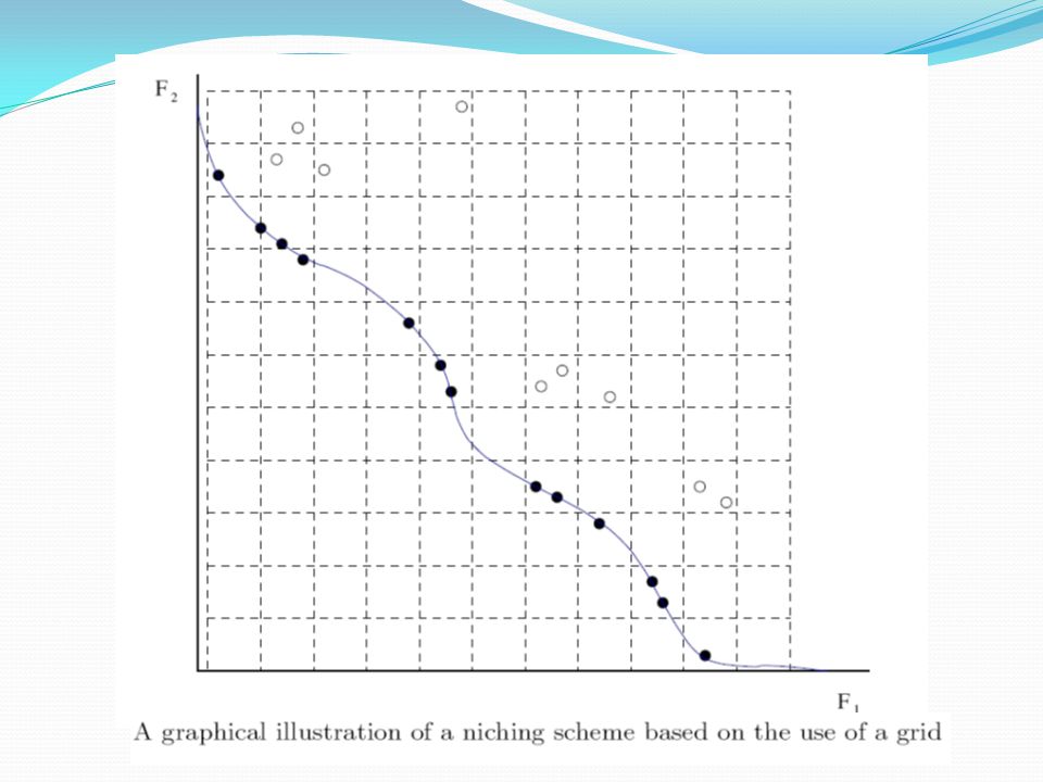
49. The Adaptive grid PAES uses a new crowding procedure based on recursively dividing up the d-dimensional objective space. This is done to minimize cost and to avoid niche-size parameter setting. Phenotype space is divided into hypercubes, which have a width of d r /2 k in each dimension, where d r is the range (maximum minus minimum) of values in objective d of the solutions currently in the archive, and k is the subdivision parameter.

50. Example grid for d=2 objectives If we use 5 levels with 2 objectives we basically have a quad-tree structure. Each level has 4 times the number of cells the previous level has. 1,4, 16, 64, 256, 1024 Hence we have 1024 regions of size (max- min)/2 5 For the simple case of k=3 the indicated cell has grid-location 101-100 or in binary 101100 0 0 1 1 Grid cell

51. So how do we find the grid location of X Recursively (for each dimension) go down the tree left (0) or right(1) creating a binary number. This requires k comparisons Then concat the binary strings creating a single binary number Note that the grid location of the previous 1024 cells is just a 10 bit string. Converting this 10 bit string to an integer gives one an index into a array Count[1024] that can be used to store the crowding number.