1. Chapter 5 The Mathematics of Diversification

2. Introduction The reason for portfolio theory mathematics:
To show why diversification is a good idea
To show why diversification makes sense logically

3. Introduction (cont’d)
Harry Markowitz’s efficient portfolios:
Those portfolios providing the maximum return for their level of risk
Those portfolios providing the minimum risk for a certain level of return

4. Introduction
A portfolio’s performance is the result of the performance of its components
The return realized on a portfolio is a linear combination of the returns on the individual investments
The variance of the portfolio is not a linear combination of component variances

5. Return
The expected return of a portfolio is a weighted average of the expected returns of the components:

6. Variance Introduction Two-security case Minimum variance portfolio
Correlation and risk reduction
The n-security case

7. Introduction
Understanding portfolio variance is the essence of understanding the mathematics of diversification
The variance of a linear combination of random variables is not a weighted average of the component variances

8. Introduction (cont’d)
For an n-security portfolio, the portfolio variance is:

9. Two-Security Case
For a two-security portfolio containing Stock A and Stock B, the variance is:

10. Two Security Case (cont’d)
Example
Assume the following statistics for Stock A and Stock B:
Stock A
Stock B
Expected return
.015
.020
Variance
.050
.060
Standard deviation
.224
.245
Weight
40%
60%
Correlation coefficient
.50

11. Two Security Case (cont’d)
Example (cont’d)
Solution: The expected return of this two-security portfolio is:

12. Two Security Case (cont’d)
Example (cont’d)
Solution (cont’d): The variance of this two-security portfolio is:

13. Minimum Variance Portfolio
The minimum variance portfolio is the particular combination of securities that will result in the least possible variance
Solving for the minimum variance portfolio requires basic calculus

14. Minimum Variance Portfolio (cont’d)
For a two-security minimum variance portfolio, the proportions invested in stocks A and B are:

15. Minimum Variance Portfolio (cont’d)
Example (cont’d)
Solution: The weights of the minimum variance portfolios in the previous case are:

16. Minimum Variance Portfolio (cont’d)
Example (cont’d)
Weight A
Portfolio Variance

17. Correlation and Risk Reduction
Portfolio risk decreases as the correlation coefficient in the returns of two securities decreases
Risk reduction is greatest when the securities are perfectly negatively correlated
If the securities are perfectly positively correlated, there is no risk reduction

18. The n-Security Case
For an n-security portfolio, the variance is:

19. The n-Security Case (cont’d)
A covariance matrix is a tabular presentation of the pairwise combinations of all portfolio components
The required number of covariances to compute a portfolio variance is (n2 – n)/2
Any portfolio construction technique using the full covariance matrix is called a Markowitz model

20. Example of Variance-Covariance Matrix Computation in Excel

23. Portfolio Mathematics (Matrix Form)
Define w as the (vertical) vector of weights on the different assets.
Define the (vertical) vector of expected returns
Let V be their variance-covariance matrix
The variance of the portfolio is thus:
Portfolio optimization consists of minimizing this variance subject to the constraint of achieving a given expected return.

24. Portfolio Variance in the 2-asset case
We have:
Hence:

25. Covariance Between Two Portfolios (Matrix Form)
Define w1 as the (vertical) vector of weights on the different assets in portfolio P1.
Define w2 as the (vertical) vector of weights on the different assets in portfolio P2.
Define the (vertical) vector of expected returns
Let V be their variance-covariance matrix
The covariance between the two portfolios is:

26. The Optimization Problem
Minimize
Subject to:
where E(Rp) is the desired (target) expected return on the portfolio and is a vector of ones and the vector is defined as:

27. Lagrangian Method
Min
Or: Min
Thus: Min

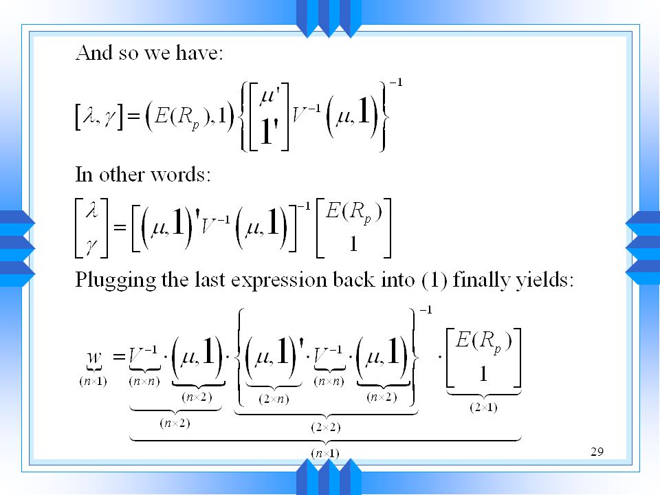
28. Taking Derivatives

30. The last equation solves the mean-variance portfolio problem
The last equation solves the mean-variance portfolio problem. The equation gives us the optimal weights achieving the lowest portfolio variance given a desired expected portfolio return.
Finally, plugging the optimal portfolio weights back into the variance
gives us the efficient portfolio frontier:

31. Global Minimum Variance Portfolio
In a similar fashion, we can solve for the global minimum variance portfolio:
The global minimum variance portfolio is the efficient frontier portfolio that displays the absolute minimum variance.

32. Another Way to Derive the Mean-Variance Efficient Portfolio Frontier
Make use of the following property: if two portfolios lie on the efficient frontier, any linear combination of these portfolios will also lie on the frontier. Therefore, just find two mean-variance efficient portfolios, and compute/plot the mean and standard deviation of various linear combinations of these portfolios.

35. Some Excel Tips
To give a name to an array (i.e., to name a matrix or a vector):
Highlight the array (the numbers defining the matrix)
Click on ‘Insert’, then ‘Name’, and finally ‘Define’ and type in the desired name.

36. Excel Tips (Cont’d)
To compute the inverse of a matrix previously named (as an example) “V”:
Type the following formula: ‘=minverse(V)’ and click ENTER.
Re-select the cell where you just entered the formula, and highlight a larger area/array of the size that you predict the inverse matrix will take.
Press F2, then CTRL + SHIFT + ENTER

37. Excel Tips (end) To multiply two matrices named “V” and “W”:
Type the following formula: ‘=mmult(V,W)’ and click ENTER.
Re-select the cell where you just entered the formula, and highlight a larger area/array of the size that you predict the product matrix will take.
Press F2, then CTRL + SHIFT + ENTER

38. Single-Index Model Computational Advantages
The single-index model compares all securities to a single benchmark
An alternative to comparing a security to each of the others
By observing how two independent securities behave relative to a third value, we learn something about how the securities are likely to behave relative to each other

39. Computational Advantages (cont’d)
A single index drastically reduces the number of computations needed to determine portfolio variance
A security’s beta is an example:

40. Portfolio Statistics With the Single-Index Model
Beta of a portfolio:
Variance of a portfolio:

41. Proof

42. Portfolio Statistics With the Single-Index Model (cont’d)
Variance of a portfolio component:
Covariance of two portfolio components:

43. Proof

44. Multi-Index Model
A multi-index model considers independent variables other than the performance of an overall market index
Of particular interest are industry effects
Factors associated with a particular line of business
E.g., the performance of grocery stores vs. steel companies in a recession

45. Multi-Index Model (cont’d)
The general form of a multi-index model: