1. Beaming

2. Beaming LHC  ~7 TeV protons   = 7000

3. 1 TeV TeV blazars

4. 10 20 eV = 10 8 TeV = 10 11 m p c 2 = tennis ball at 100 km/s Cosmic rays

5. A few milligrams per decade?

6. Radio-loud AGNs Gamma Ray Bursts ~ 0.1 M o yr -1  ~20 ~ 10 -5 M o in a few sec  ~300

7. Lorentz transformations: v along x x’ =  (x – vt) y’ = y z’ = z t’ =  (t – v x/c 2 ) for  t = 0   x =  x’/  Contraction for  x’ = 0   t =  t’ time dilation Text book special relativity x =  (x’ + vt’) y = y’ z = z’ t =  (t’ + v x’/c 2 ) To remember: mesons created at a height of ~15 km can reach the earth, even if their lifetime is a few microsec  ct’ life =hundreds of meters.

8. v=0  =1 v=0.866c  =2 v Can we see contracted spheres? Einstein: Yes!

9. James Terrel 1959 Roger Penrose 1959 v=0  =1 v NO! v=0.866c  =2 Rotation, not contraction!

10. Relativity with photons From rulers and clocks to photographs and frequencies Or: from elementary particles to extended objects

11. The moving square  =0  =0.5 Your camera, very far away

12. The moving square t=l’/c vt=  l’ l’/  l tot = l’ (  +1/  ) max:2 1/2 l’ (diag) min: l’ (for  =0)

13. l’ l’cos  =  l’  cos  =  cos  sin  

14.  ) 

15. 

16. Time CD = c  t e – c  t e  cos    t A =  t e (1-  cos  )   t A =  t e ’  (1-  cos  )  t e = emission time in lab frame  t e ’ = emission time in comov. frame  t e =  t e ’ 

17. Relativistic Doppler factor   t A =  t e ’  (1-  cos  )  t A =  t e ’  (1-  cos  ) = ’ /  (1-  cos  ) = ’ /  (1-  cos  )  =  =1  (1-  cos  )  (1-  cos  ) Standard relativity Doppler effect You change frame You remain in lab frame

18. Relativistic Doppler factor  = = = =1  (1-  cos  )  (1-  cos  ) 2  for  =0 o  for  =1/   for   =  At small angles, Doppler wins over Spec. Relat.

19. 2 5 l i g h t y e a r s i n 3 y e a r s … t h e v e l o c i t y i s 8. 3 c

20. Nucleo v=0.99c

21. Core

22.  app =  sin  1-  cos   =  v app = v   t e  sin   t e (1-  cos  )  s app tAtAtAtA  =0 o   app =0 cos  =  ; sin  =1/    app =   =90 o   app =  There is no  Correct?

23.  app ~ 30

24. Aberration of light

25. Gravity bends space

26. Aberration of light sin  = sin  ’/  d  =  d  ’/  2

27. sin  = sin  ’/  Aberration of light K’ d  = d  ’/  2 K v

28. Observed vs intrinsic Intensity  3 I’( ’) I( )  I’( ’) ’  ’  = =invariant I( ) = cm 2 s Hz sterad =erg= dA dt d d  E

29. Observed vs intrinsic Intensity  3 I’( ’) I( )  I’( ’) ’  ’  = =invariant I( ) = cm 2 s Hz sterad =erg= dA dt d d  E

30. Observed vs intrinsic Intensity  3 I’( ’) I( )  I’( ’) ’  ’  = =invariant I( ) = cm 2 s Hz sterad =erg= dA’ d  ’/  2 E’   3 I’( ’) = I  4 I’ = F  4 F’ =

31. v=0 L=100 W

32. v= 0.995 c  =10 L=16MW L=10mW L=0.6mW

33. v= 0.995 c  =10 blazars radiogalaxies …….?

34. v= 0.995 c  =10 blazars radiogalaxies blazars!

35. jet counterjet (invisible) v v

36. A question Some blob is moving at  >>1, above a black hole of mass M. It is optically thin. It moves within a region full of radiation produced by the accretion disk. What is the Eddington luminosity? 

37. U rad U’ rad ~  2 U rad Little help….

38. Radiation processes

39.  Line emission and radiative transitions in atoms and molecules  Breemstrahlung/Blackbody  Curvature radiation  Cherenkov  Annihilation  Unruh radiation  Hawking radiation  Synchrotron  Inverse Compton

40. V=0 V=0 E

41. () V (  =2 ) Charge at time 9.00 Contracted sphere… E-field lines at time 9.00 point to… where the charge is at 9.00 E Breaking news: what happens with the gravitational field?

42. dP = e 2 a 2 sin 2  d  4  c 3 V http://www.cco.caltech.edu/~phys1/java/phys1/MovingCharge/MovingCharge.html Stop at 8:00

43. Synchrotron

44. Synchrotron  Ingredients: Magnetic field and relativistic charges  Responsible: Lorentz force  Curiously, the Lorentz force doesn’t work. FL =FL =FL =FL =ddt (  mv) =ec v x B 

45. Total losses P e = P’ e Please, P e is not P received !! P=E/t and E and t Lorentz transform in the same way

46. Total losses a’ =  3 a a’ =  2 a P e = P’ e = 2e 2 3c 3 (  2 a 2 + a 2 ) 4444 2e 2 = 3c 3 a’ 2 = 2e 2 3c 3 (a’ 2 + a’ 2 ) P e = P’ e Big? NO! a is small Why?

47. FL =FL =FL =FL =ddt (  mv) =ec v x B a || = 0 a = e v B sin   mc P S (  ) = 2e 4 3m 2 c 3  B 2   2  2 sin 2  P S (  ) = 2  T  cU B   2  2 sin 2  r 0 =e 2 /m e c 2  T = 8  r 0 /3 2 = = 4  T cU B   2  2 3 If pitch angles are isotropic  =pitch angle  ~constant, at least for one gyroradius

48. FL =FL =FL =FL =ddt (  mv) =ec v x B a || = 0 a = e v B sin   mc P S (  ) = 2e 4 3m 2 c 3  B 2   2  2 sin 2  P S (  ) = 2  T  cU B   2  2 sin 2  r 0 =e 2 /m e c 2  T = 8  r 0 /3 2 = = 4  T cU B   2  2 3 If pitch angles are isotropic

49. Log E Log P S v 2 ~ E   ~ E 2 Why  2 ?? P S (  ) = 2  T  U B   2  2 sin 2  What happens when   0 ? Sure, but what happens to the received power if you are in the beam of the particles?

50.  mc 2  sin  eB rLrLrLrL = v2v2v2v2a = e B  mc = B = 1/T T = 2  r L /v = 1/T T = 2  r L /v Synchrotron Spectrum Characteristic frequency This is not the characteristic frequency e v B sin   mc a =

51. v<<c v ~ c

52.  t A = ?

53. S = S = 1 tAtAtAtA = 2222eB 2  mc  Compare with B. S = B  3

54. The real stuff x= x 1/3

55. The real stuff x=

56. Emission from many particles N(  ) = K  -p The queen of relativistic distributions Log N(  ) Log  Log Log   )  ( ) d  = 1 4444 N(  ) P S d 

57. Emission from many particles N(  ) = K  -p The queen of relativistic distributions Log N(  ) Log  Log Log   )  ( )  ~ 1 4444 K  -p B 2  2 d  d Emission is peaked!  Emission is peaked!  S= 2222eB 2  mc dddd d

58. Emission from many particles N(  ) = K  -p The queen of relativistic distributions Log N(  ) Log  Log Log   )  ( )  ~ 1 4444 K B 2 (2-p)/2 -1/2 B 1/2 B (2-p)/2

59. Emission from many particles N(  ) = K  -p The queen of relativistic distributions Log N(  ) Log  Log Log   )  ( )  ~ 1 4444 K B (1+p)/2 (1-p)/2

60. Emission from many particles N(  ) = K  -p The queen of relativistic distributions Log N(  ) Log  Log Log   )  ( )  ~ 1 4444 K B  +1 -  ====p-12 power law

61.  ( )  ~ 1 4444 K B  +1 -  So, what? 4  Vol  ( ) ~  s 2 R K B  +1 -  F( ) ~ 4d24d24d24d2 Log Log F  ) K B  +1 If you know  s and R Two unknowns, one equation… we need another one

62. Synchrotron self-absorption If you can emit you can also absorbIf you can emit you can also absorb Synchrotron is no exceptionSynchrotron is no exception With Maxwellians it would be easy (Kirchhoff law) to get the absorption coefficientWith Maxwellians it would be easy (Kirchhoff law) to get the absorption coefficient But with power laws?But with power laws? Help: electrons able to emit are also the ones that can absorbHelp: electrons able to emit are also the ones that can absorb

63. A useful trick  -p Many Maxwellians with kT=  mc 2 I( ) = 2 kT 2 /c 2 = 2  mc 2 2 /c 2 Log  Log N(  = 2222eB 2  mc  B) 1/2  ~ (  B) 1/2 5/2 5/2 B 1/2 ~ There is no K !

64. From data to physical parameters get B insert B and get K t belongs to thick and thin part. Then in principle one observation is enough

65. Inverse Compton

66. Scattering is one the basic interactions between matter and radiation.Scattering is one the basic interactions between matter and radiation. At low photon frequencies it is a classical process (i.e. e.m. waves)At low photon frequencies it is a classical process (i.e. e.m. waves) At low frequencies the cross section is called the Thomson cross section, and it is a peanut.At low frequencies the cross section is called the Thomson cross section, and it is a peanut. At high energies the electron recoils, and the cross section is the Klein-Nishina one.At high energies the electron recoils, and the cross section is the Klein-Nishina one.

67.  = scattering angle 0 1 Thomson scattering hv 0 << m e c 2 hv 0 << m e c 2 tennis ball against a wall tennis ball against a wall The wall doesn’t move The wall doesn’t move The ball bounces back with the same speed (if it is elastic) The ball bounces back with the same speed (if it is elastic) 1 = 0 1 = 0

68. Thomson cross section dTdTdTdT dddd = r0r0r0r022 (1+cos 2  ) TTTT = r0r0r0r0 2 3 8888 = r0r0r0r0 mec2mec2mec2mec2 e2e2e2e2 a peanut Electromagnetic mass of the electron: See Vol. 2, chapter 28.3 of The Feynman Lectures on Physics

69. Why a peanut?

71. E B

72. d dd ddP e2a2e2a2e2a2e2a2 4  c 3 sin 2  = Remember:

73. E B

74. dTdTdTdT dddd = r0r0r0r022 (1+cos 2  ) 1 2 100% Pol no Pol

75. Direct Compton x1 =x1 =x1 =x1 = x0x0x0x0 1+x 0 (1-cos  ) x = h mec2mec2mec2mec2  x0x0x0x0 x1x1x1x1 Klein-Nishina cross section

77. ~ E -1 Klein-Nishina cross section

78. Inverse Compton: typical frequencies Thomson regime Rest frame K’ x’ 1 =x’ x x’ x1x1x1x1 Lab frame K

79. Min and max frequencies  = 180 o  1 =0 o x 1 =4  2 x  = 0 o  1 =180 o x 1 =x/4  2

80. Total loss rate vt TTTT Everything in the lab frame n(  ) = density of seed photons of energy  =h n(  ) = density of seed photons of energy  =h v rel = “relative velocity” between photon and electron v rel = c-vcos  c(1-  cos  )

81. Total loss rate vt TTTT There are many  1, because there are many  1.. We must average the term 1-  cos  1, getting

82. Total loss rate There are many  1, because there are many  1.. We must average the term 1-  cos  1, getting Then U rad {

83. Total loss rate If seed are isotropic, average over  and take out the power of the incoming radiation, to get the net electron losses: U rad { = = 4  T cU rad   2  2 3 = = 4  T cU B   2  2 3 Compare with synchrotron losses:

84. If the seeds are not isotropic….

86. Inverse Compton spectrum The typical frequency is:          Going to the rest frame of the e- we see  0  There the scattered radiation is isotropized  Going back to lab we add another  -factor.

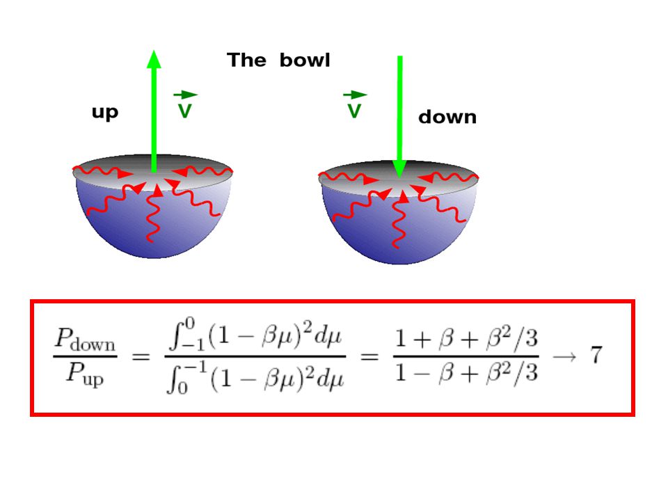
87. The real stuff downupscattering

88. downupscattering 75%

89. Emission from many particles N(  ) = K  -p The queen of relativistic distributions Log N(  ) Log  Log Log   )  ( ) d  = 1 4444 N(  ) P C d 

90. Emission from many particles N(  ) = K  -p The queen of relativistic distributions Log N(  ) Log  Log Log   )  ( )  ~ 1 4444 K  -p U rad  2 d  d Emission is peaked!  Emission is peaked!  dddd d4 =  2 0 3

91. Emission from many particles N(  ) = K  -p The queen of relativistic distributions Log N(  ) Log  Log Log   )  ( )  ~ 1 4444 KU rad (2-p)/2 -1/2

92. Emission from many particles N(  ) = K  -p The queen of relativistic distributions Log N(  ) Log  Log Log   )  ( )  ~ 1 4444 KU rad -  ====p-12 power law

93. Synchrotron Self Compton: SSC Due to synchro, then proportional to:  c B  +1 -   c ( ) ~  2 c B  +1 c -   2 c B  +1 c -  Electrons work twice

95. End ?

96. World records  Frequency??  1/t Planck ~ 10 43 Hz, but…  Power??  M Planck c 2 /t Planck ~ 3.6x10 59 erg/s

97. End

104. The moving bar

105. =0=0=0=0