1. A Multiperiod Production Problem
Example 3.3
A Multiperiod Production Problem

2. Background Information
The Pigskin Company produces footballs.
Pigskin must decide how many footballs to produce each month. It has decided to use a 6-month planning horizon.
The forecasted demands for the next 6 months are 10,000, 15,000, 30,000, 35,000, 25,000 and 10,000.
Pigskin wants to meet these demands on time, knowing that it currently has 5000 footballs in inventory and that it can use a given month’s production to help meet the demand for that month.

3. Background Information -- continued
During each month there is enough production capacity to produce up to 30,000 footballs, and there is enough storage capacity to store up to 10,000 footballs at the end of the month, after demand has occurred.
The forecasted production costs per football for the next 6 months are $12.50, $12.55, $12.70, $12.80, $12.85, and $12.95, respectively.
The holding cost per football held in inventory at the end of the month is figured at 5% of the production cost for that month.

4. Background Information -- continued
The selling price for footballs is not considered relevant to the production decision because Pigskin will satisfy all customer demand exactly when it occurs – at whatever the selling price is.
Therefore Pigskin wants to determine the production schedule that minimizes the total production and holding costs.

5. Solution
In the traditional algebraic formulation, the decision variables are the production quantities for the 6 months, labeled P1 through P6.
It is convenient to let I1 through I6 be the corresponding end-of-month inventories(after the demand has occurred).
For example, I3 is the number of footballs left over at then end of month 3. Therefore, the obvious constraints are on production and inventory storage capacities: Pj  300 and Ij  100 for each month j, 1  j  6.

6. Solution -- continued
In addition to these constraints, we need balance constraints that relate the P ’s and I ’s.
In any month the inventory from the previous month plus the current production must equal the current demand plus leftover inventory.
If Dj is the forecasted demand for month j, then the balance equation for month j is Ij-1 + Pj = Dj + Ij.

7. Solution -- continued
The first of these constraints, for month j = 1, uses the known beginning inventory, 50, for the previous inventory (the Ij-1 term)
By putting all variables (P’s and I’s) on the left and all known values on the right (a standard LP convention), these balance constraints become
P1 – I1 =
I1 + P2 – I2 = 150
I2 + P3 – I3 = 300
I3 + P4 – I4 = 350
I4 + P5 – I5 = 250
I5 + P6 – I6 = 100

8. Solution -- continued
As usual, we impose nonnegativity constraints. All P’s and I’s must be nonnegative.What about meeting demand on time?
This requires that in each month the inventory from the preceding month plus the current production must be at least as large as the current demand.
Finally, the objective is the sum of unit production costs multiplied by P’s, plus unit holding costs multiplied by I’s.

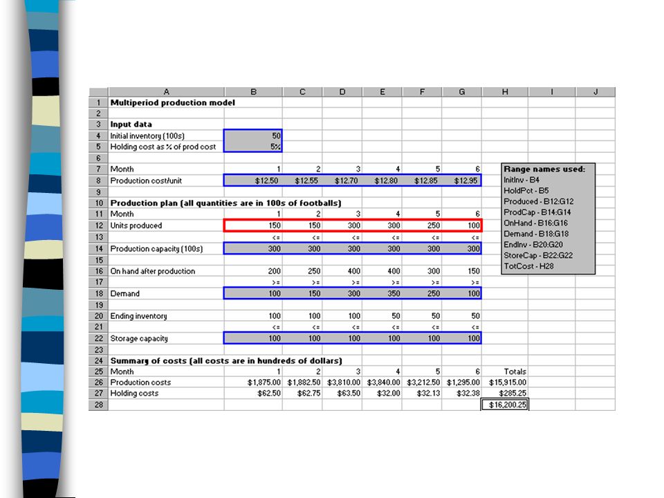
9. PIGSKIN.XLS
This file shows the spreadsheet model of Pigskin’s production problem.
The spreadsheet figure on the next slide shows the model.

11. Developing the Model
The main feature that distinguishes this model from the product mix model is that some of the constraints, namely, the balance constraints, are built into the spreadsheet itself by means of formulas.
In other words, the only changing cells are the production quantities.
The ending inventories shown in row 20 are determined by the production quantities and equations.

12. Developing the Model -- continued
To form the spreadsheet model in proceed as follows.
Inputs. Enter the inputs in the shaded ranges. Again, these are all entered as numbers straight from the problem statement.
Production quantities. Enter any values in the range Produced as the production quantities. As always, you can enter values that you believe are good, maybe even optimal.
On-hand inventory. Enter the formula =InitInv + B12 in cell B16. This calculates the first month on-hand inventory after production. Then enter the “typical” formula =B20 + C12 for on-hand inventory after production in month 2 in cell C16 and copy it across row 16.

13. Developing the Model -- continued
Ending inventories. Enter the formula =B16 – B18 for ending inventory in cell B20 and copy it to the rest of the EndInv range. This formula calculates ending inventory in the current month as on-hand inventory before demand minus the demand in that month.
Production and holding costs. Enter the formula =B8 * B12 in cell B26 and copy it across to cell G27 to calculate the monthly holding costs.Note that these are based on monthly ending inventories. Finally, calculate the cost totals in column H by summing with the SUM function.

14. Developing the Model -- continued
The logic behind the constraints is now straightforward.
All we have to guarantee is that
The production quantities are nonnegative and do not exceed the production capacities.
The on-hand inventories after production are at least as large as demands.
Ending inventories do not exceed storage capacities.

15. Developing the Model -- continued
Using the Solver – To use the Solver, fill out the dialog boxes as follows and then click on Solve.
Model. Fill out the Solver dialog box as shown below.

16. Developing the Model -- continued
Options. In the Solver Options dialog box, check the Assume Linear Model and Assume Non-Negative boxes.
The Solver solution appears on the next slide.
This solution is also represented graphically on the following slide.
We can interpret the solution by comparing production quantities with demands.

19. Interpreting the Solution
In month 1 Pigskin should produce just enough to meet month 1 demand.
In month 2 it should produce 5000 more footballs than month 2 demand, and then in month 3 it should produce just enough to meet month 3 demand, still carrying the extra 5000 footballs in inventory from month 2 production.
In month 4 Pigskin should finally use these footballs, along with the maximum production amount, 30,000, to meet month 4 demand.
Then in months 5 and 6 it should produce exactly enough to meet these months’ demands.

20. Interpreting the Solution -- continued
The total cost is $1,535,563, most of which is production cost.
Could you have guessed that this is the optimal solution?
Upon some reflection, it makes perfect sense. Because the monthly holding costs are large relative to the differences in monthly production costs, there is little incentive to produce footballs before they are needed to take advantage of a “cheap”production month.

21. Interpreting the Solution -- continued
Therefore, the Solver tells us to produce footballs in the month in which they are needed – when this is possible.
The only exception to this rule is the 20,000 footballs produced during month 2 when only 15,000 are needed.
The extra 5000 units produced during month 2 are needed, however, to meet month 4’s demand of 35,000, because month 3 production capacity is used entirely to meet month 3 demand. Thus month 3 capacity is not available to meet month 4 demand, and 5000 units of month 2 capacity are used to meet month 4 demand.

22. Sensitivity Analysis
We can use the SolverTable add-in to perform a number of interesting sensitivity analyses.
We illustrate two possibilities.
First, note that the most inventory we ever carry at the end of the month is 50, although the storage capacity each month is 100. Perhaps this is because the holding cost percentage, 5% is fairly large.
Would we carry more ending inventory if this holding cost percentage were reduced? Or would we carry less if it were increased?

23. Sensitivity Analysis -- continued
We check this with the SolverTable output shown here.

24. Sensitivity Analysis -- continued
Now the single input cell is the HoldPct cell, and the single output we keep track of is the maximum ending inventory ever held, which we calculate in cell B31 with the formula =MAC(EndInv) in cell B32.
As we see, only when the holding cost percentage decreases to 1% do we reach the storage capacity limit.
On the other side, even when the holding cost percentage reaches 10%, we still continue to hold a maximum ending inventory of 50.

25. Sensitivity Analysis -- continued
A second possible sensitivity analysis is suggested by the way the optimal production schedule would probably be implemented.
The optimal solution to Pigskin’s model specifies the production level for each of the next 6 months.
In reality, however, the company might implement the model’s recommendation only for the first month.
Then at the beginning of the second month, it will gather new forecasts for the next 6 months, months 2 and 7, solve a new 6-month model, and again implement the model’s recommendation for the first of these months, month 2.

26. Sensitivity Analysis -- continued
If the company continues in this manner, we say that it is following a 6-month rolling planning horizon.
The question then is whether the assumed demands toward the end of the planning horizon have much effect on the optimal production quantity in month 1.
We would hope not because these forecasts could be inaccurate.

27. Sensitivity Analysis -- continued
The two-way Solver table shown here shows how the optimal month 1 production quantity varies with the assumed demands in months 5 and 6.

28. Sensitivity Analysis -- continued
As we see, if assumed month 5 and 6 demands remain fairly small, the optimal month 1 production quantity remains at 50.
It means that the optimal production quantity in month 1 is fairly insensitive to the possibly inaccurate forecasts for months 5 and 6.