Download presentation
Presentation is loading. Please wait.

1
Fast Fourier Transform for speeding up the multiplication of polynomials an Algorithm Visualization Alexandru Cioaca

2
Defining the problem

3
The explicit form of a polynomial is given by the list of coefficients and we can use it to compute the polynomial’s values at any point (for any variable) This operation is called Evaluation In reverse, if we have the values of a polynomial of order N at at least N distinct points, we can determine its coefficients This operation is called Interpolation
 This operation is called Evaluation In reverse, if we have the values of a polynomial of order N at at least N distinct points, we can determine its coefficients This operation is called Interpolation")
4
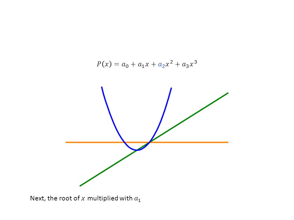
Consider the following polynomial

9
Adding these 4 components gives us our polynomial (in black)
")
10
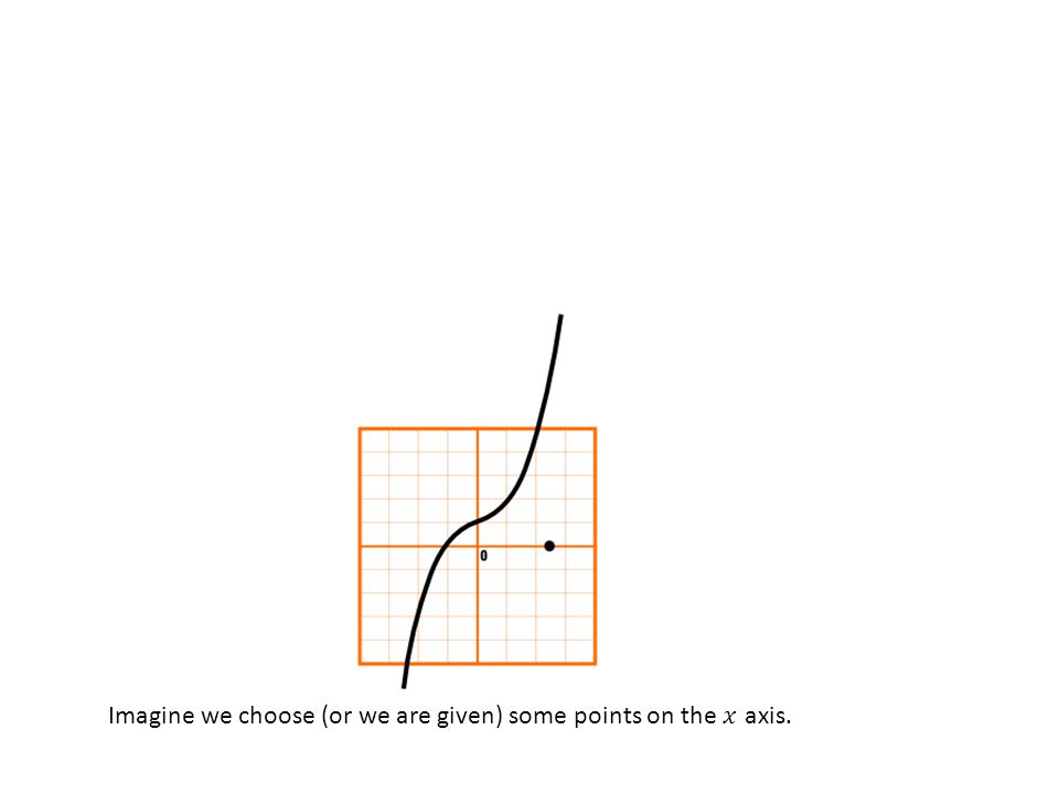
Let’s draw a cartesian grid for our polynomial

14
We can evaluate our polynomial at these points. This is Evaluation.

15
Now imagine the reverse operation for our polynomial. What if we don’t have its explicit form, so we can’t evaluate it?

16
Instead, we only have its value at certain points.

17
From these values, the polynomial can be reconstructed approximately. This approximation is better for more and more values.

18
This is Interpolation.

20
Consider the following two polynomials Their product is

21
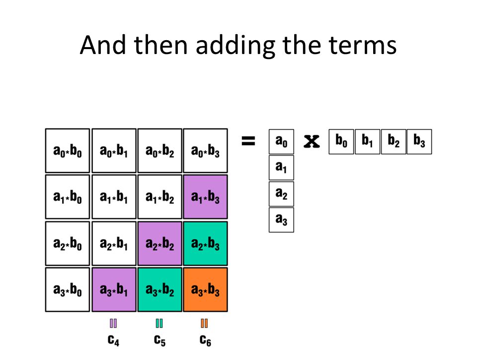
The coefficients of the product polynomial can be computed from the following outer-product

22
This means computing the product of each pair of coefficients

26
And then adding the terms

32
Look at the symmetry of these roots on the Unit Circle

33
N=1

34
N=2

35
N=3

36
N=4

37
N=5

38
N=6

39
N=7

40
N=8

42
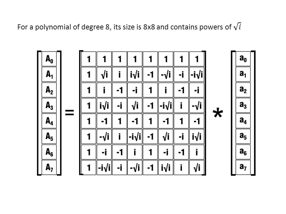
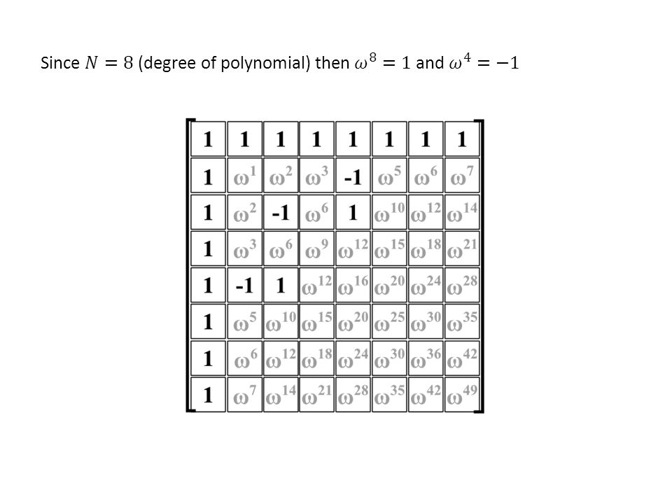
We can see the DFT matrix is a Vandermonde matrix of the Nth roots of unity

44
The rows of the DFT matrix correspond to basic harmonic waveforms They transform the seed vector in the spectral plane

45
This computation is nothing but a matrix-vector product

46
Each element of the result is equal to the inner product of the corresponding row of the matrix with the seed vector

47
So we are dealing with 8 terms obtained from multiplications

48
Adding these terms that come from multiplications

49
And, first and foremost, computing the elements of the DFT matrix..

50
..for every pair of elements from the matrix and the vector

52
Because we have to do this for each row. Which might be take a while..

53
We can speed up the matvec using some nice properties of DFT This is the FFT algorithm (FAST Fourier Transform)
")
65
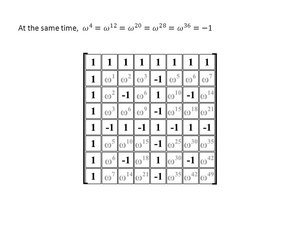
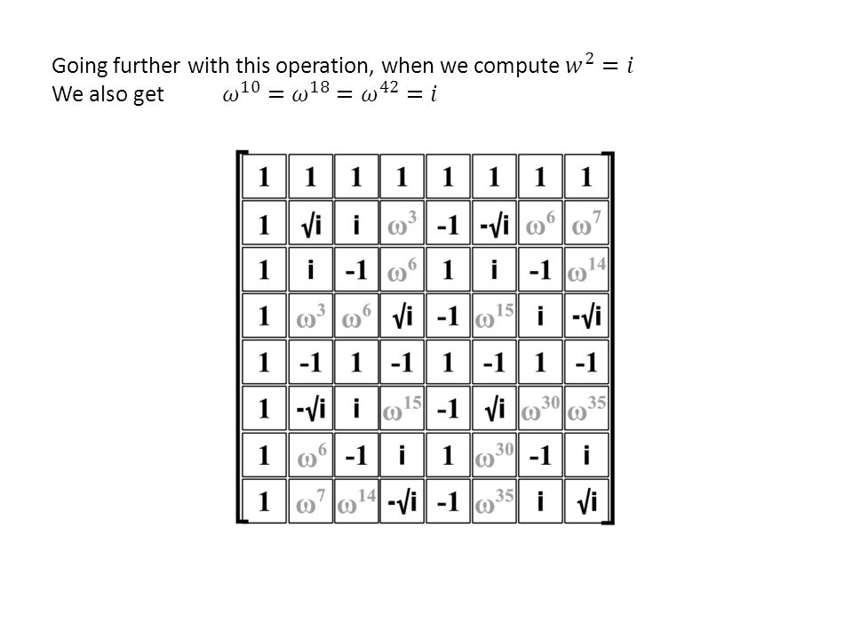
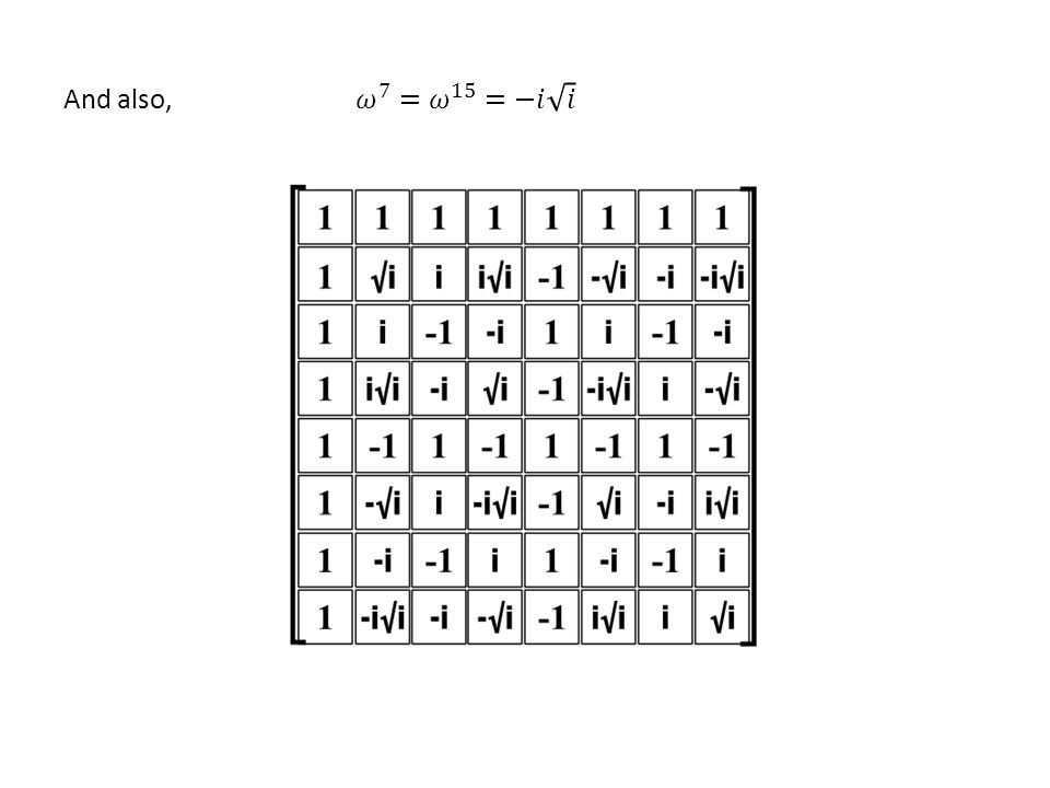
Only after 3-4 steps, we filled the DFT matrix completely

66
FFT is used to compute this matrix-vector product with a smaller number of computations. It is a recursive strategy of divide-and-conquer. FFT uses the observation made previously that we can express any polynomial as a sum between its terms in odd coefficients and those in even coefficients. This operation can be repeated until we split the polynomial in linear polynomials that can be easily evaluated Fast Fourier Transform (FFT)
.")
67
FFT

68
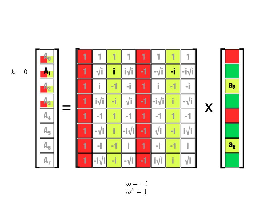
FFT transforms the vector of coefficients “a” into the vector “A”.

69
FFT It starts by splitting the given vector of coefficients in two subvectors. One contains the odd-order coefficients, and the other one contains those of even order.

70
FFT Then, it proceeds in a recursive fashion to split these vectors again

71
FFT This recursion stops when we reach subvectors of degree 1

72
FFT The actual computation is performed when the algorithm starts to exit the recursion.

73
FFT At each step backward, the output coefficients are updated.

74
FFT It evaluates polynomials from the

75
Let’s follow the algorithm step-by-step on the DFT matrix-vector product.

76
We pass the vector of coefficients to FFT which starts the recursion

77
First, it splits the 8 coefficients in 2 sets (odd and even)
")
78
It follows the recursion down one step for the first set of coefficients.

79
FFT splits this vector too and the recursion goes down one more step.

80
At the third split (log 8 = 3), FFT is passed a linear polynomial and returns.
, FFT is passed a linear polynomial and returns.")
81
FFT reached a polynomial of order 1, so it will evaluate it.

82
The first coefficient of A gets updated with this value.

83
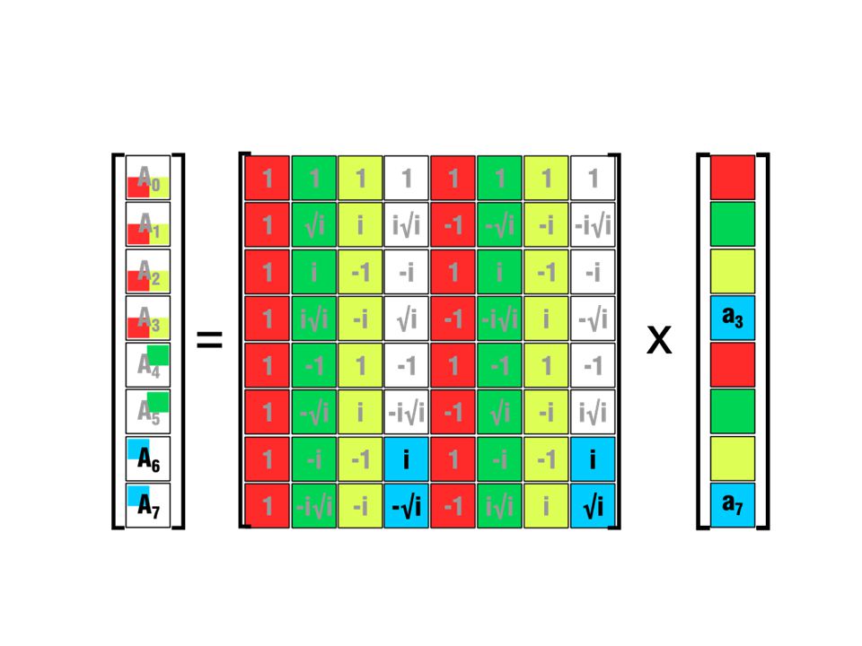
Then, FFT evaluates the polynomial at the negative of the previous root.

84
The corresponding coefficient is updated with this value.

85
By computing these two values, FFT already computed the pairs for the other 3 polynomials.

86
We now exit the FFT for this polynomial (RED) and enter the branch of the recursion corresponding to the next polynomial
 and enter the branch of the recursion corresponding to the next polynomial")
87
Again, we evaluate the two values.

88
And update the corresponding coefficients.

89
Looking at the corresponding columns, we can see that the other values are computed, but can be used only when the other polynomials are active, and when FFT evaluates at the right power of the primitive root of unity

90
After exiting the recursion to the second level, we can update the output coefficients by interchanging the values computed already.

93
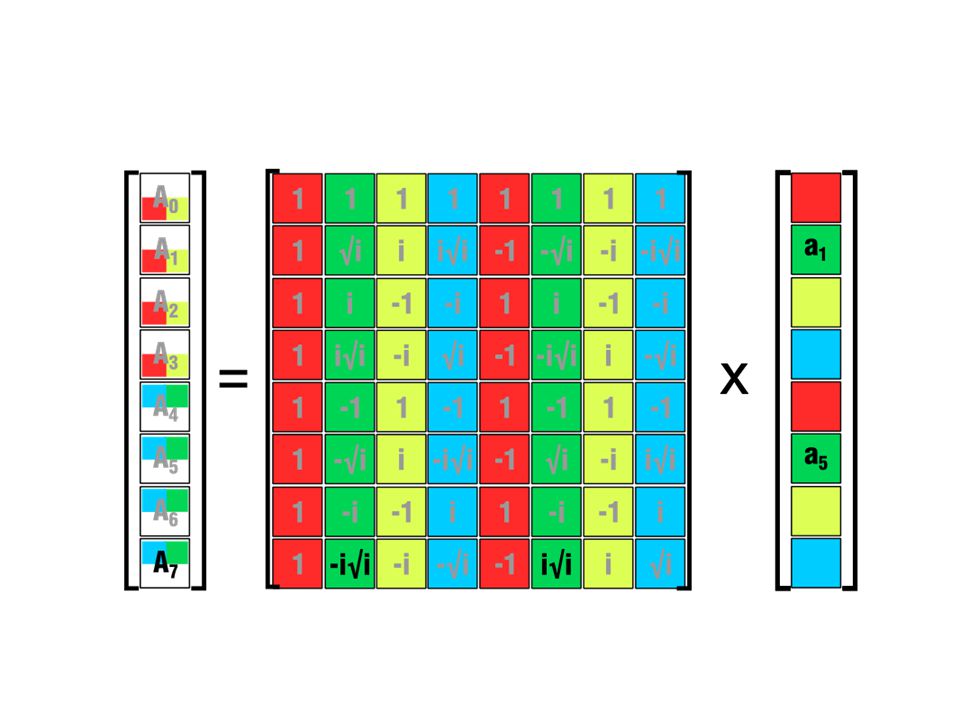
FFT exits the recursion to the higher level and works on the second half.

94
FFT evaluates these basic polynomials too, and updates the coefficients.

98
After evaluating the last linear polynomial, FFT has computed all the values it needs. From now on, the computation will rely on combining these values.

99
Exiting the recursion, the coefficients are, again, updated at each step.

104
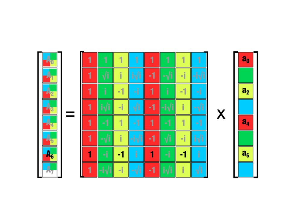
Finally, FFT goes back to the upper level and combines the subpolynomials.

105
At this level, we can see the strength of FFT.

106
It combines larger subpolynomials, so the computation is being sped up exponentially with each level.

111
With FFT, after three levels of recursion, we computed the matvec product.

113
Multiplying the polynomials In order to compute the product-polynomial, we will have to evaluate the two polynomials at enough points (2n-1) and multiply them element-wise These products correspond to the spectral coefficients of the product. In order to obtain its explicit form, we have to interpolate these values. This is done with the inverse DFT matrix, which contains the inverse of the DFT matrix, taken element-wise. We can employ the same FFT algorithm to compute this fast.

Similar presentations


 The Discrete Fourier Transform.>")


 These lecture.>")
 Lecture 16: Application-Driven Hardware Acceleration (1/4)>")


