1. Global Sequence Alignment by Dynamic Programming

2. Needleman-Wunsch Algorithm General Algorithm for sequence comparison Maximize a similarity score to give the maximum match Maximum match=largest number of amino acids or nucleotides of one sequence that can be matched with another, allowing for all possible deletions.

3. Needleman-Wunsch Algorithm Finds the best GLOBAL alignment of any two sequences. N-M involves an iterative matrix method of calculation All possible pairs (nucleotides or amino acids) are represented in a two- dimensional array. All possible alignments are represented by pathways through this array.

4. Needleman-Wunsch Algorithm Sequence alignment methods predate dot- matrix searches, and all of the alignment methods in use today are related to the original method of Needleman and Wunsch (1970). Needleman and Wunsch wanted to quantify the similarity between two sequences.

5. Needleman-Wunsch Algorithm Over the course of evolution, some positions undergo base or amino acid substitutions, and bases or amino acids can be inserted or deleted. Any measurement of similarity must therefore be done with respect to the best possible alignment between two sequences. Because insertion/deletion events are rare compared to base substitutions, it makes sense to penalize gaps more heavily than mismatches when calculating a similarity score.

6. Dynamic Programming Finding the best alignment of 2 sequences is a hard problem solved by a computational method called dynamic programming Multiple sequence alignment of 3 or more sequences can be solved by dynamic programming and statistical methods

7. How Do We Generate the Correct Alignment ? We can't. We can never guarantee that a particular alignment is correct except for the simplest, unambiguous alignments! Such an alignment would require aligning each sequence in turn to the ancestral sequence first. Since there is no possibility to know the ancestral sequence and the evolutionary steps, the evolutionary correctness of any alignment cannot be determined.

8. The Optimal Alignment. If the optimal alignment does not support homology, then the correct alignment (which has a smaller or equal score) will not support homology either. But again: there is no guarantee that the optimal alignment is the correct alignment, even though it may be the best guess.

9. Dynamic Programming Dynamic programming is a term from operations research, where it was first used to describe a class of algorithms for the optimization of dynamic systems.

10. Dynamic Programming In dynamic programming the principle of divide-and-conquer is used extensively: subdivide a problem that is to large to be computed, into smaller problems that may be efficiently computed. Then assemble the answers to give a solution for the large problem. When you do not know which smaller problem to solve, simply solve all smaller problems, store the answers and assembled them later to a solution for the large problem.

11. Dynamic Programming Global optimal alignment is a difficult problem. The major difficulty comes from the fact, that one cannot simply slide one sequence along another and sum over the similarity scores looked up in the appropriate mutation data matrix. This will not work, because biological sequences may have gaps or insertions of sequences relative to each other.

12. Three steps in Dynamic Programming 1. Initialization 2 Matrix fill or scoring 3. Traceback and alignment

13. Sample Matrix To align with a cell in the diagonal means an alignment in the next position. An increasing diagonal line means a stretch of sequence identity. To align with an off-diagonal cell requires the insertion of a corresponding number of gaps.

14. Needleman-Wunsch Algorithm We can compute for every cell the highest possible score that can be obtained for a path originating from that cell. That is done by looking in all the elements permissible for extending the path, and adding the highest value found to the contents of the cell.

15. Needleman-Wunsch Algorithm If this is done in an orderly way, the highest score found is the global maximum alignment score. Then the optimal path consists of all those cells that contributed to the global maximum alignment score. There can be several equivalent optimal paths.

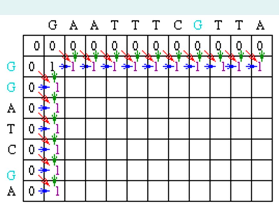
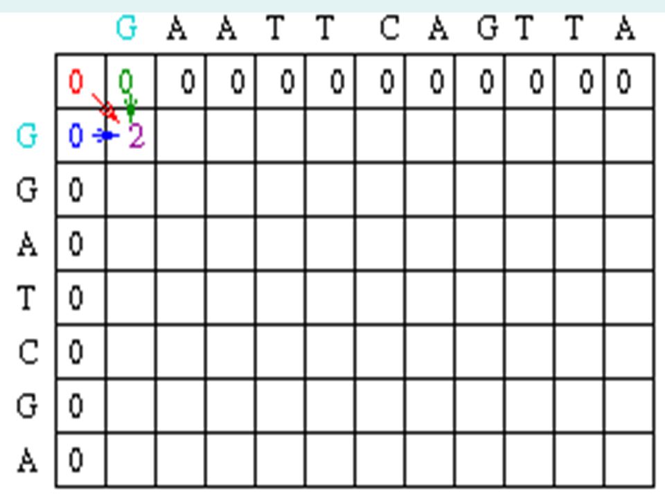
16. Sample Matrix Create a matrix with M + 1 columns and N + 1 rows where M and N correspond to the size of the sequences to be aligned. Since this example assumes there is no gap opening or gap extension penalty, the first row and first column of the matrix can be initially filled with 0.

20. Matrix Fill Step One possible solution of the matrix fill step finds the maximum global alignment score by starting in the upper left hand corner in the matrix and finding the maximal score Mi,j for each position in the matrix. In order to find Mi,j for any i,j it is minimal to know the score for the matrix positions to the left, above and diagonal to i, j. In terms of matrix positions, it is necessary to know Mi-1,j, Mi,j-1 and Mi-1, j-1.

21. Matrix Fill Step In the example, Mi-1,j-1 will be red, Mi,j-1 will be green and Mi-1,j will be blue. Since the gap penalty (w) is 0, the rest of row 1 and column 1 can be filled in with the value 1.

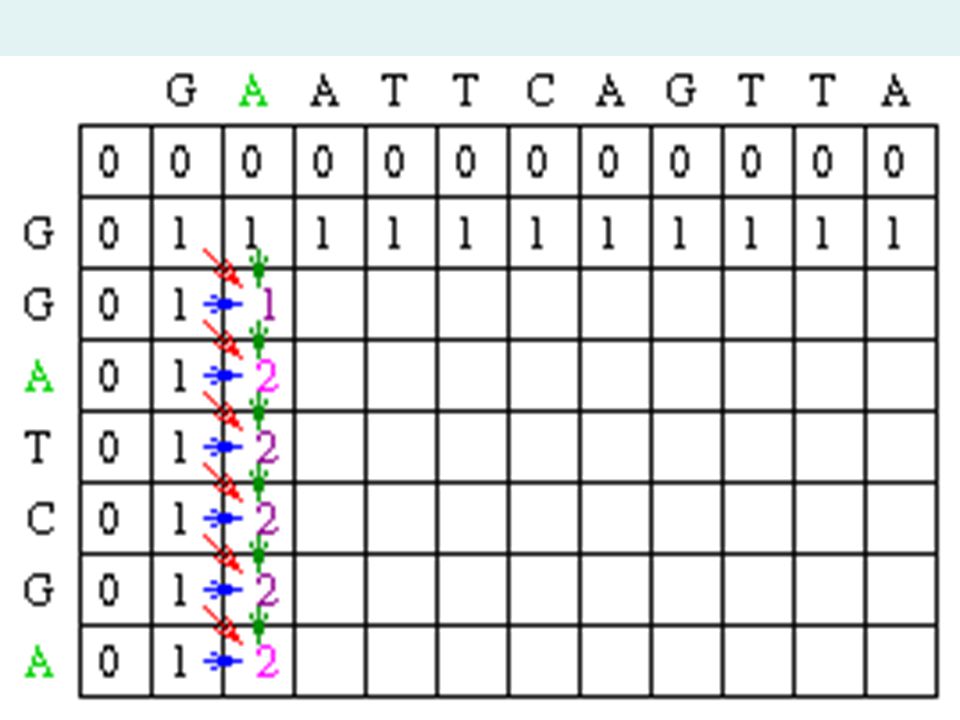
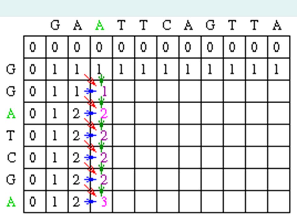
23. Matrix Fill Step Now let's look at column 2. The location at row 2 will be assigned the value of the maximum of 1(mismatch), 1(horizontal gap) or 1 (vertical gap). So its value is 1. At the position column 2 row 3, there is an A in both sequences. Thus, its value will be the maximum of 2(match), 1 (horizontal gap), 1 (vertical gap) so its value is 2.

27. Traceback Step After the matrix fill step, the maximum alignment score for the two test sequences is 6. The traceback step determines the actual alignment(s) that result in the maximum score. With a simple scoring algorithm like this one, there are likely to be multiple maximal alignments. The traceback step begins in the M,J position in the matrix- the position that leads to the maximal score. In this case, there is a 6 in that location.

28. Traceback Step Traceback takes the current cell and looks to the neighbor cells that could be direct predecessors. This means it looks to the neighbor to the left (gap in sequence #2), the diagonal neighbor (match/mismatch), and the neighbor above it (gap in sequence #1). The algorithm for traceback chooses as the next cell in the sequence one of the possible predecessors. The neighbors are marked in red and are also equal to 5.

32. Traceback Step Since the current cell has a value of 6 and the scores are 1 for a match and 0 for anything else, the only possible predecessor is the diagonal match/mismatch neighbor. If more than one possible predecessor exists, any can be chosen.

33. Traceback Step This gives us a current alignment of (Seq #1) A | (Seq #2) A So now we look at the current cell and determine which cell is its direct predecessor. In this case, it is the cell with the red 5.

35. This is One Traceback Giving an alignment of : G A A T T C A G T T A | | | | | | G G A _ T C _ G _ _ A

37. This is an alternative Traceback giving an alignment of : G _ A A T T C A G T T A | | | | | | G G _ A _ T C _ G _ _ A

38. What Is the Best Alignment Between These Two Amino Acid Sequences? A zinc-finger core sequence: CKHVFCRVCI A sequence fragment from a viral protein: CKKCFCKCV

39. Practice Matrix C K H V F C R V C I +-------------------- C | K | C | F | C | K | C | V |

40. Place a 1 Where There Is a Match in the Matrix C K H V F C R V C I +-------------------- C | 1 1 1 K | 1 C | 1 1 1 F | 1 C | 1 1 1 K | 1 C | 1 1 1 V | 1 1

41. Place Zeroes on the Ends Since They Can’t Align C K H V F C R V C I +-------------------- C | 1 1 1 0 K | 1 0 C | 1 1 1 0 F | 1 0 C | 1 1 1 0 K | 1 0 C | 1 1 1 0 V | 0 0 0 1 0 0 0 1 0 0

42. Loading the Matrix Then proceed to the next row and column, adding to each matrix cell the maximal value of any other cell that could be the next step on a path to the matrix. For instance the value 1 at (C6,C8) now becomes a 2, since it could be extended from the 1 at (V8,V9) through a 1.

44. C K H V F C R V C I +-------------------- C | 1 1 1 0 K | 1 0 0 C | 1 1 1 0 F | 1 0 0 C | 1 1 1 0 K | 1 0 0 C | 2 1 1 1 1 2 1 0 1 0 V | 0 0 0 1 0 0 0 1 0 0 Filling the Matrix

45. C K H V F C R V C I +-------------------- C | 1 1 1 1 0 K | 1 1 0 0 C | 1 1 1 1 0 F | 1 1 0 0 C | 1 1 1 1 0 K | 2 3 2 2 2 1 1 1 0 0 C | 2 1 1 1 1 2 1 0 1 0 V | 0 0 0 1 0 0 0 1 0 0 Repeat This Procedure for the Next Row and Column:

46. And the Next … C K H V F C R V C I +-------------------- C | 1 1 1 1 1 0 K | 1 1 1 0 0 C | 1 1 1 1 1 0 F | 1 1 1 0 0 C | 4 2 2 2 2 2 1 1 1 0 K | 2 3 2 2 2 1 1 1 0 0 C | 2 1 1 1 1 2 1 0 1 0 V | 0 0 0 1 0 0 0 1 0 0

47. And the Next Row… C K H V F C R V C I +-------------------- C | 1 2 1 1 1 0 K | 1 1 1 1 0 0 C | 1 2 1 1 1 0 F | 3 2 2 2 3 1 1 1 0 0 C | 4 2 2 2 2 2 1 1 1 0 K | 2 3 2 2 2 1 1 1 0 0 C | 2 1 1 1 1 2 1 0 1 0 V | 0 0 0 1 0 0 0 1 0 0

48. And the Next … C K H V F C R V C I +-------------------- C | 1 2 2 1 1 1 0 K | 1 2 1 1 1 0 0 C | 4 3 3 3 2 2 1 1 1 0 F | 3 2 2 2 3 1 1 1 0 0 C | 4 2 2 2 2 2 1 1 1 0 K | 2 3 2 2 2 1 1 1 0 0 C | 2 1 1 1 1 2 1 0 1 0 V | 0 0 0 1 0 0 0 1 0 0

49. And the Next … C K H V F C R V C I +-------------------- C | 1 3 2 2 1 1 1 0 K | 1 3 2 1 1 1 0 0 K | 3 4 3 3 2 1 1 1 0 0 C | 4 3 3 3 2 2 1 1 1 0 F | 3 2 2 2 3 1 1 1 0 0 C | 4 2 2 2 2 2 1 1 1 0 K | 2 3 2 2 2 1 1 1 0 0 C | 2 1 1 1 1 2 1 0 1 0 V | 0 0 0 1 0 0 0 1 0 0

50. And the Next … C K H V F C R V C I +-------------------- C | 1 3 3 2 2 1 1 1 0 K | 4 4 3 3 2 1 1 1 0 0 K | 3 4 3 3 2 1 1 1 0 0 C | 4 3 3 3 2 2 1 1 1 0 F | 3 2 2 2 3 1 1 1 0 0 C | 4 2 2 2 2 2 1 1 1 0 K | 2 3 2 2 2 1 1 1 0 0 C | 2 1 1 1 1 2 1 0 1 0 V | 0 0 0 1 0 0 0 1 0 0

51. Another Path Marked C K H V F C R V C I +-------------------- C | 5 3 3 3 2 2 1 1 1 0 K | 4 4 3 3 2 1 1 1 0 0 K | 3 4 3 3 2 1 1 1 0 0 C | 4 3 3 3 2 2 1 1 1 0 F | 3 2 2 2 3 1 1 1 0 0 C | 4 2 2 2 2 2 1 1 1 0 K | 2 3 2 2 2 1 1 1 0 0 C | 2 1 1 1 1 2 1 0 1 0 V | 0 0 0 1 0 0 0 1 0 0

52. Filling the Matrix The globally optimal score is the highest score in the first row or column - for the N- terminus of either protein sequence. In our example it is 5. Therefore, the globally optimal alignment will have 5 matches. Let us now back trace our path ending at the cell with value 5 to see how we arrived at the value. Strip away all the cells that could not have contributed to the sum.

53. C K H V F C R V C I +-------------------- C | 5 K | 4 K | 4 3 3 C | 3 3 F | 3 C | 2 K | 2 1 1 C | 2 1 1 V | 1 There are several equally good paths to a score of 5

54. A Number of Different Alignments Are Possible: C K H V F C R V C I C K K C F C - K C V C K H V F C R V C I C K K C F C K - C V C - K H V F C R V C I C K K C - F C - K C V C K H - V F C R V C I C K K C - F C - K C V

55. Advanced Dynamic Programming An advanced scoring scheme is assumed where –Si,j = 2 if the residue at position i of sequence #1 is the same as the residue at position j of sequence #2 (match score); otherwise –Si,j = -1 (mismatch score) –w = -2 (gap penalty)

56. Adding Gaps and Mismatches The second A-G pair is a mismatch. G A A T T C A G T T A | | | | | | G G A T _ C _ G _ _ A The fifth T has no pair so this is a gap. Or it could be an insertion or gain of sequence.

57. Creating the Matrix The first step in the global alignment dynamic programming approach is to create a matrix with M + 1 columns and N + 1 rows where M and N correspond to the size of the sequences to be aligned. The first row and first column of the matrix can be initially filled with 0.

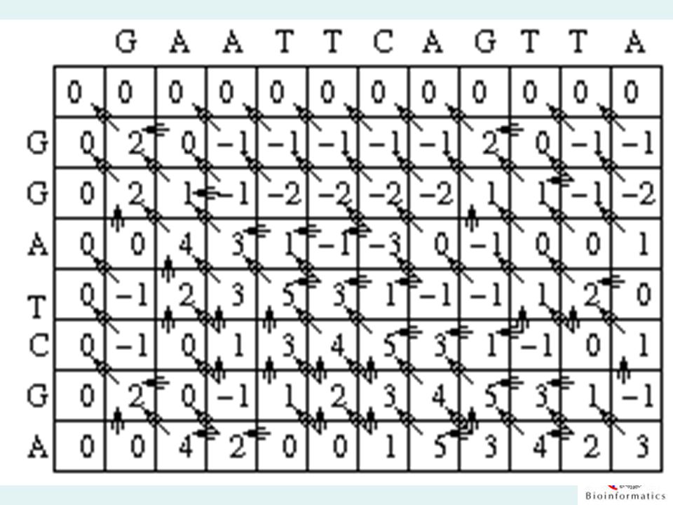
58. Creating the Matrix For each position, Mi,j is defined to be the maximum score at position i,j; i.e. Mi,j = MAXIMUM[ Mi-1, j-1 + Si,j (match/mismatch in the diagonal), Mi,j-1 + w (gap in sequence #1), Mi-1,j + w (gap in sequence #2)] Note that in the example, Mi-1,j-1 will be red, Mi,j-1 will be green and Mi-1,j will be blue

60. Moving down the first column to row 2, we can see that there is once again a match in both sequences. Thus, S1,2 = 2. So M1,2 = MAX[M0,1 + 2, M1,1 - 2, M0,2 -2] = MAX[0 + 2, 2 - 2, 0 - 2] = MAX[2, 0, -2]. A value of 2 is then placed in position 1,2 of the scoring matrix and an arrow is placed to point back to M[0,1] which led to the maximum score.

62. Filling the Matrix Looking at column 1 row 3, there is not a match in the sequences, so S 1,3 = -1. M1,3 = MAX[M0,2 - 1, M1,2 - 2, M0,3 - 2] = MAX[0 - 1, 2 - 2, 0 - 2] = MAX[-1, 0, -2]. A value of 0 is then placed in position 1,3 of the scoring matrix and an arrow is placed to point back to M[1,2] which led to the maximum score.

64. Eventually, we get to column 3 row 2. Since there is not a match in the sequences at this position, S3,2 = -1. M3,2 = MAX[ M2,1 - 1, M3,1 - 2, M2,2 - 2] = MAX[0 - 1, -1 - 2, 1 -2] = MAX[-1, - 3, -1]. So you begin to get loss of scores.

66. Filling the Matrix and Using Pointers Note that in the above case, there are two different ways to get the maximum score. In such a case, pointers are placed back to all of the cells that can produce the maximum score.

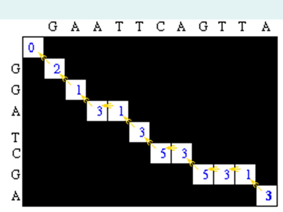
69. Traceback This gives an alignment of G A A T T C A G T T A | | | | | | G G A _ T C _ G _ _ A

71. Traceback This gives another alignment of G A A T T C A G T T A | | | | | | G G A T _ C _ G _ _ A

72. Gap Penalty The gap penalty is used to help decide whether on not to accept a gap or insertion in an alignment when it is possible to achieve a good alignment residue-to-residue at some other neighboring point in the sequence. You need a penalty, because an unreasonable 'gappy' alignment would result. Biologically, it should in general be easier for a protein to accept a different residue in a position, rather than having parts of the sequence chopped away or inserted.

73. Gap Penalty Gaps/insertions should therefore be more rare than point mutations (substitutions). Some different possibilities: –A single gap-open penalty. This will tend to stop gaps from occurring, but once they have been introduced, they can grow unhindered. –A gap penalty proportional to the gap length. This will work against larger gaps. –A gap penalty that combines a gap-open value with a gap-length value.

74. Substitution Matrix A substitution matrix describes the likelihood that two residue types would mutate to each other in evolutionary time. This is used to estimate how well two residues of given types would match if they were aligned in a sequence alignment.

75. Substitution Matrix An amino acid substitution matrix is a symmetrical 20*20 matrix, where each element contains the score for substituting a residue of type i with a residue of type j in a protein, where i and j are one of the 20 amino-acid residue types. Same residues should obviously have high scores, but if we have different residues in a position, how should that be scored?

76. Substitution Matrix Scoring The same residues in a position give the score value 1, and different residues give 0. The same residues give a score 1, similar residues (for example: Tyr/Phe, or Ile/Leu) give 0.5, and all others 0. One may calculate, using well established sequence alignments, the frequencies (probabilities) that a particular residue in a position is exchanged for another.

77. Substitution Matrix Scoring This was done originally be Margaret Dayhoff, and her matrices are called the PAM (Point Accepted Mutation) matrices, which describe the exchange frequencies after having accepted a given number of point mutations over the sequence. Typical values are PAM 120 (120 mutations per 100 residues in a protein) and PAM 250. There are many other substitution matrices: BLOSUM, Gonnet, etc.

78. Scoring Similarity 1) Can only score aligned sequences 2) DNA is usually scored as identical or not 3) Modified scoring for gaps - single vs. multiple base gaps (gap extension) 4) AAs have varying degrees of similarity –a. # of mutations to convert one to another –b. chemical similarity –c. observed mutation frequencies 5) PAM matrix calculated from observed mutations in protein families

79. The PAM 250 Scoring Matrix

80. GCG Wisconsin Package GAP GAP is the implementation of the Needleman- Wunsch algorithm in the GCG program package. The NW algorithm will present you with a single globally optimal alignment, not all possible optimal alignments - different alignments may exist that give the same score. GAP presents you with one member of the family of best alignments that align the full length of one sequence to the full length of a second sequence. There may be many members of this family, but no other member has a higher score.

81. GCG Wisconsin Package GAP The primary use of a global alignment algorithm is when you really want the whole of two sequences to be aligned, without truncation. GAP could completely bypass a region of high local homology, if a better (or even just as good) path can be found in a different way. This is problematic if one short sequence is aligned against a longer one with internal repeats. If there is weak or unknown similarity between two sequences, a local alignment algorithm (BESTFIT) is the better choice. Use GAP only when you believe the similarity is over the whole length.

82. Limitations to Needleman- Wunsch The problem with Needleman-Wunsch is the amount of processor memory resources it requires. Because of this, it is not favored for practical use, despite the guarantee of an optimal alignment. The other difficulty is that the concept of global alignment is not used in pairwise sequence comparison searches.