1. Statistical tests for Quantitative variables (z-test & t-test) BY Dr.Shaikh Shaffi Ahamed Ph.D., Associate Professor Dept. of Family & Community Medicine College of Medicine, King Saud University

2. Choosing the appropriate Statistical test Based on the three aspects of the data Types of variables Number of groups being compared & Sample size

3. Statistical Tests Z-test: Study variable: Qualitative Outcome variable: Quantitative or Qualitative Comparison: Sample mean with population mean & sample proportion with population proportion; two sample means or two sample proportions Sample size: larger in each group(>30) & standard deviation is known Student’s t-test: Study variable: Qualitative Outcome variable: Quantitative Comparison: sample mean with population mean; two means (independent samples); paired samples. Sample size: each group <30 ( can be used even for large sample size)

4. Test for sample proportion with population proportion In an otological examination of school children, out of 146 children examined 21 were found to have some type of otological abnormalities. Does it confirm with the statement that 20% of the school children have otological abnormalities? a. Question to be answered: Is the sample taken from a population of children with 20% otological abnormality b. Null hypothesis : b. Null hypothesis : The sample has come from a population with 20% otological abnormal children Problem

5. c. Test statistics d.Comparison with theoritical value Z ~ N (0,1); Z 0.05 = 1.96 The prob. of observing a value equal to or greater than 1.69 by chance is more than 5%. We therefore do not reject the Null Hypothesis e. Inference There is a evidence to show that the sample is taken from a population of children with 20% abnormalities Test for sample prop. with population prop. P – Population. Prop. p- sample prop. n- number of samples

6. Comparison of two sample proportions In a community survey, among 246 town school children, 36 were found with conductive hearing loss and among 349 village school children 61 were found with conductive hearing loss. Does this data, present any evidence that conductive hearing loss is as common among town children as among village children? Problem

7. Comparison of two sample proportions a. Question to be answered: Is there any difference in the proportion of hearing loss between children living in town and village? Given data sample 1 sample 2 size 246 342 hearing loss 36 61 % hearing loss 14.6 % 17.5% b. Null Hypothesis There is no difference between the proportions of conductive hearing loss cases among the town children and among the village children

8. Comparison of two sample proportions c. Test statistics p1, p2 are sample proportions, n1,n2 are subjects in sample 1 & 2 q= 1- p

9. Comparison of two sample proportions d. Comparison with theoretical value Z ~ N (0,1); Z 0.05 = 1.96 The prob. of observing a value equal to or greater than 1.81 by chance is more than 5%. We therefore do not reject the Null Hypothesis e. Inference There is no evidence to show that the two sample proportions are statistically significantly different. That is, there is no statistically significant difference in the proportion of hearing loss between village and town, school children.

10. Comparison of two sample means Example : Weight Loss for Diet vs Exercise Diet Only: sample mean = 5.9 kg sample standard deviation = 4.1 kg sample size = n = 42 standard error = SEM 1 = 4.1/  42 = 0.633 Exercise Only: sample mean = 4.1 kg sample standard deviation = 3.7 kg sample size = n = 47 standard error = SEM 2 = 3.7/  47 = 0.540 Did dieters lose more fat than the exercisers? measure of variability = [(0.633) 2 + (0.540) 2 ] = 0.83

11. Example : Weight Loss for Diet vs Exercise Step 1. Determine the null and alternative hypotheses. The sample mean difference = 5.9 – 4.1 = 1.8 kg and the standard error of the difference is 0.83. Null hypothesis: No difference in average fat lost in population for two methods. Population mean difference is zero. Alternative hypothesis: There is a difference in average fat lost in population for two methods. Population mean difference is not zero. Step 2. Sampling distribution: Normal distribution (z-test) Step 3. Assumptions of test statistic ( sample size > 30 in each group) Step 4. Collect and summarize data into a test statistic. So the test statistic: z = 1.8 – 0 = 2.17 0.83

12. Example : Weight Loss for Diet vs Exercise Step 5. Determine the p-value. Recall the alternative hypothesis was two-sided. p-value = 2  [proportion of bell-shaped curve above 2.17] Z-test table => proportion is about 2  0.015 = 0.03. Step 6. Make a decision. The p-value of 0.03 is less than or equal to 0.05, so … If really no difference between dieting and exercise as fat loss methods, would see such an extreme result only 3% of the time, or 3 times out of 100. Prefer to believe truth does not lie with null hypothesis. We conclude that there is a statistically significant difference between average fat loss for the two methods.

13. Student’s t-test 1.Test for single mean Whether the sample mean is equal to the predefined population mean ?. Test for difference in means 2. Test for difference in means Whether the CD4 level of patients taking treatment A is equal to CD4 level of patients taking treatment B ? Test for paired observation 3. Test for paired observation Whether the treatment conferred any significant benefit ?

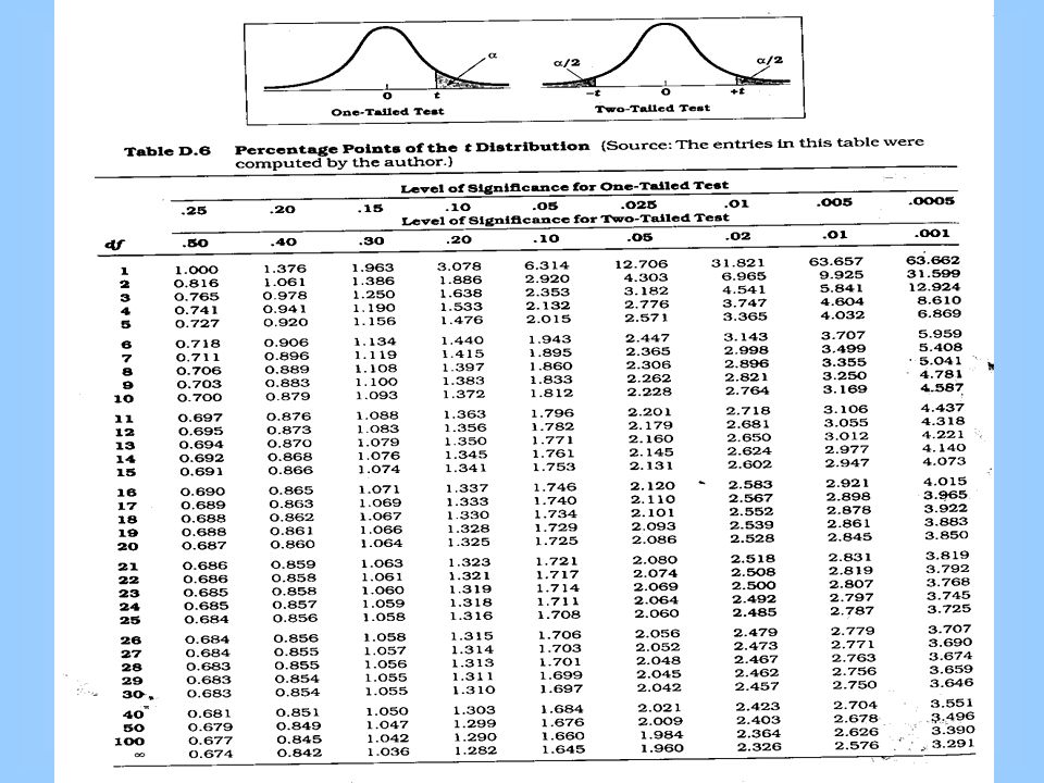
14. Steps for test for single mean 1.Questioned to be answered Is the Mean weight of the sample of 20 rats is 24 mg? N=20, =21.0 mg, sd=5.91, =24.0 mg 2. Null Hypothesis The mean weight of rats is 24 mg. That is, The sample mean is equal to population mean. 3. Test statistics --- t (n-1) df 4. Comparison with theoretical value if tab t (n-1) < cal t (n-1) reject Ho, if tab t (n-1) > cal t (n-1) accept Ho, 5. Inference

15. t –test for single mean Test statistics n=20, =21.0 mg, sd=5.91, =24.0 mg t  = t.05, 19 = 2.093 Accept H 0 if t = 2.093 Inference : We reject Ho, and conclude that the data is not providing enough evidence, that the sample is taken from the population with mean weight of 24 gm

17. Given below are the 24 hrs total energy expenditure (MJ/day) in groups of lean and obese women. Examine whether the obese women’s mean energy expenditure is significantly higher ?. Lean 6.1 7.0 7.5 7.5 5.5 7.6 7.9 8.1 8.1 8.1 8.4 10.2 10.9 t-test for difference in means Obese Obese 8.8 9.2 9.2 8.8 9.2 9.2 9.7 9.7 10.0 9.7 9.7 10.0 11.5 11.8 12.8 11.5 11.8 12.8

18. Null Hypothesis Obese women’s mean energy expenditure is equal to the lean women’s energy expenditure. Data Summary lean Obese N 13 9 8.10 10.30 S 1.38 1.25

19. H 0 :  1 -  2 = 0 (  1 =  2 ) H 1 :  1 -  2  0 (  1   2 )  = 0.05 df = 13 + 9 - 2 = 20 Critical Value(s): t 02.086-2.086.025 Reject H 0 0.025 Solution

20. t XX S nSnS nn dfnn P              1212 211 2 22 2 12 1 2 11 11 2  Hypothesized Difference (usually zero when testing for equal means) Compute the Test Statistic: ()) ( ()() ()() n1n1 n2n2 __ Calculating the Test Statistic:

21. Developing the Pooled-Variance t Test Calculate the Pooled Sample Variances as an Estimate of the Common Populations Variance: = Pooled-Variance = Variance of Sample 1 = Variance of sample 2 = Size of Sample 1 = Size of Sample 2

22. S nSnS nn P              2 11 2 22 2 12 22 11 11 131 1 3891125 13 1 91 1 765... (( (( ( ( ( ( ) ) ) ) ) )) ) First, estimate the common variance as a weighted average of the two sample variances using the degrees of freedom as weights

23. t XX S nn P      1212 2 12 10.3 0 176 1 + 13 1919 3.82  8.1. Calculating the Test Statistic: ( (())) tab t 9+13-2 =20 dff = t 0.05,20 =2.086

25. T-test for difference in means Inference : The cal t (3.82) is higher than tab t at 0.05, 20. ie 2.086. This implies that there is a evidence that the mean energy expenditure in obese group is significantly (p<0.05) higher than that of lean group

26. Computing the Independent t-test Using SPSS Enter data in the data editor or download the file. Click analyze  compare means  independent sample t-test. The independent samples t-test dialog box should open. Click on the independent variable, and click the arrow to move it to the grouping variable box. Highlight the variable (? ?) in the grouping variable box. Click define groups. Enter the value 1 for group 1 and 2 for group 2. Click continue. Click on the dependent variable, and click the arrow to place it in the test variable(s) box.

27. Interpreting the Output The group statistics box provides the mean, standard deviation, and number of participants for each group (level of the IV).

28. Interpreting the Output Levene’s test is designed to compare the equality of the error variance of the dependent variable between groups. We do not want this result to be significant. If it is significant, we must refer to the bottom t-test value. t is your test statistic and Sig. is its two-tailed probability. If testing a one-tailed hypothesis, we need to divide this value in half. df provides the degrees of freedom for the test, and mean difference provides the average difference in scores/values between the two groups.

29. Example Suppose we want to test the effectiveness of a program designed to increase scores on the quantitative section of the Graduate Record Exam (GRE). We test the program on a group of 8 students. Prior to entering the program, each student takes a practice quantitative GRE; after completing the program, each student takes another practice exam. Based on their performance, was the program effective?

30. Each subject contributes 2 scores: repeated measures design StudentBefore ProgramAfter Program 1520555 2490510 3600585 4620645 5580630 6560550 7610645 8480520

31. Can represent each student with a single score: the difference (D) between the scores Student Before ProgramAfter Program D 152055535 249051020 3600585-15 462064525 558063050 6560550-10 761064535 848052040

32. Approach: test the effectiveness of program by testing significance of D Null hypothesis: There is no difference in the scores of before and after program Alternative hypothesis: program is effective → scores after program will be higher than scores before program → average D will be greater than zero H 0 : µ D = 0 H 1 : µ D > 0

33. Student Before Program After ProgramDD2D2 1520555351225 249051020400 3600585-15225 462064525625 5580630502500 6560550-10100 7610645351225 8480520401600 ∑D = 180∑D 2 = 7900 So, need to know ∑D and ∑D 2 :

34. Recall that for single samples: For related samples: where: and

35. Standard deviation of D: Mean of D: Standard error:

36. Under H 0, µ D = 0, so: From Table B.2: for α = 0.05, one-tailed, with df = 7, t critical = 1.895 2.714 > 1.895 → reject H 0 The program is effective.

38. Computing the Paired Samples t-test Using SPSS Enter data in the data editor or open the file. Click analyze  compare means  paired samples t-test. The paired samples t-test dialog box should open. Hold down the shift key and click on the set of paired variables (the variables representing the data for each set of scores). Click the arrow to move them to the paired variables box. Click OK.

39. Interpreting the Output The paired samples statistics box provides the mean, standard deviation, and number of participants for each measurement time. The test statistic box provides the mean difference between the two test times, the t-ratio associated with this difference, its two-tailed probability (Sig.), and the degrees of freedom associated with the design. As with the independent t-test, if testing a one-tailed hypothesis, divide the significance level in half.

40. Z- value & t-Value “Z and t” are the measures of: How difficult is it to believe the null hypothesis? High z & t values Difficult to believe the null hypothesis - accept that there is a real difference. Low z & t values Easy to believe the null hypothesis - have not proved any difference.

41. In conclusion ! Z-test will be used for both categorical(qualitative) and quantitative outcome variables. Student’s t-test will be used for only quantitative outcome variables.