1. RF Networks

2. There are two aspects of networking which must be considered when installing either an NCL or LMS product:
1. Ethernet Networking (IP)
2. Radio Networking (RF)
This presentation will focus on the RF side of the NCL and LMS products.

3. RF Terminology
Wavelength is the distance between identical points in the adjacent cycles of a waveform. In wireless systems, this length is usually specified in meters, centimeters, or millimeters

4. At 2.4 GHz the wavelength is 12.5cm
The size of the wavelength varies depending on the frequency of the signal. Generally speaking, the higher the frequency the smaller the wavelength.
The WaveRider family of products operate in the GHz range (NCL and LMS2000) as well as the MHz range (LMS3000).
At 2.4 GHz the wavelength is 12.5cm
At 905 MHz the wavelength is 33cm

5. These values are calculated using the following formula:
Wavelength = 3 x 102
f (frequency in MHz)
This calculation is important to remember, especially when installing antennas. Ideally, the antenna should be installed no closer than 10 wavelengths to the nearest reflective surface.

6. Frequency Kilohertz (kHz) Megahertz (MHz) Gigahertz (GHz)
Frequency is the number of complete cycles per second in alternating current direction. The standard unit of frequency is the hertz, abbreviated Hz. If a current completes one cycle per second, then the frequency is 1 Hz.
Kilohertz (kHz)
Megahertz (MHz)
Gigahertz (GHz)
Terahertz (THz)
Audio 20 Hz to 20 KHz
FM radio band 88 MHz to 108 MHz
North American cellular 824 MHz to 896 MHz
National Paging 929 MHz MHz
North American PCS 1850 MHz to 1990 MHz

7. Frequency Spectrum Basic resource for wireless communications
practical radio communication between 3 KHz and 300 GHz
new systems designed tend to go higher in frequency providing larger bandwidth

8. Spectrum Mobile bands Upper part of band for base Tx
lower part of band for base Rx

9. Tx Power Tx is short for “Transmit”
All radios have a certain level or Tx power that the radio generates at the RF interface. This power is calculated as the amount of energy given across a defined bandwidth and is usually measured in one of two units:
dBm – a relative power level referencing 1 milliwatt
W – a linear power level referencing Watts

10. dBm = 10 x log[Power in Watts / 0.001W]
W = x 10[Power in dBm / 10 dBm]
The NCL and LMS radios have Tx power of +18dBm, which translates into .064 W or 64 mW.

11. Rx Sensitivity Rx is short for “Receive”
All radios also have a certain ‘point of no return’, where if they receive a signal less than the stated Rx Sensitivity, the radio will not be able to ‘see’ the data.
This is also stated in dBm or W.
The NCL and LMS radios have a receive sensitivity of –82 dBm. At this level, a Bit Error Rate (BER) of 10-5 (99.999%) is seen.
The actual level received at the radio will vary depending on many factors.

12. Radiated Power dBi: relative to an isotropic radiator
In a wireless system, antennas are used to convert electrical waves into electromagnetic waves. The amount of energy the antenna can ‘boost’ the sent and received signal by is referred to as the antennas Gain.
Antenna gain is measured in:
dBi: relative to an isotropic radiator
dBd: relative to a dipole radiator
0 dBd = 2.15 dBi

13. There are certain guidelines set by the FCC that must be met in terms of the amount of energy radiated out of an antenna. This ‘energy’ is measured in one of two ways:
Effective Isotropic Radiated Power (EIRP)
measured in dBm = power at antenna input [dBm] + relative antenna gain [dBi]
Effective Radiated Power (ERP)
measured in dBm = power at antenna input [dBm] + relative antenna gain [dBd]

14. Energy Losses
In all wireless communication systems there are several factors that contribute to the loss of signal strength. Cabling, connectors, lightning arrestors can all impact the performance of your system if not installed properly.
In a ‘low power’ system (such as the NCL and LMS products) every dB you can save is important!! Remember the “3 dB Rule”.
For every 3 dB gain/loss you will either double your power (gain) or lose half your power (loss).

15. -3 dB = 1/2 power
-6 dB = 1/4 power
+3 dB = 2x power
+6 dB = 4x power
Sources of loss in a wireless system: free space, cables, connectors, jumpers, obstructions

16. FCC Guidelines The ISM Bands are defined as follows: 902 to 928 MHz
FCC Part 15, Class B
Unlicensed operation from to MHz
P2P - EIRP : +36 dBm (4 Watts)
: 3:1 i.e. +24 dBm into 24 dBi
P2MP - EIRP : +36 dBm (4 Watts)
: 3:1 at subscriber (considered P2P)

17. FCC - Installer
System must be installed by a “Professional Installer” as defined in FCC Document Part 15;
Complete understanding of FCC emissions regulations for unlicensed operation in the 2.4 GHz ISM Band.
Installer must have a full understanding of the impact of various types of antennae, amplifiers and other active and passive components on the compliance of the equipment under FCC regulations.

18. FCC - Installation
An external Power Amp cannot be used in conjunction with WR radio components, in order to comply with FCC regulatory emissions requirements. Use of an external PA device with a WaveRider system is deemed illegal and may result in significant penalty to the manufacturer, seller, and customer.
Unique connectors provide means of compliance.
Standard connectors require professional installation to ensure compliance.

19. WaveRider High Speed Wireless Systems
The NCL and LMS systems are designed to support terrestrial fixed links in an outdoor environment. Typical distances achieved while staying within FCC guidelines are:
Point to Multipoint: up to 8km
Point to Point: up to 15km
These distances may vary depending on the installation, antennae chosen, cabling, etc.

20. NCL1155 Spec Sheet

21. Direct Sequence Spread Spectrum
Also known as Direct Sequence Code Division Multiple Access (DS-CDMA), DSSS is one of two approaches to spread spectrum modulation for digital signal transmission over the air.
The stream of information to be transmitted is divided into small pieces, each of which is allocated to a frequency channel across the spectrum.
When transmitted, the data is combined with a higher data-rate bit sequence (also known as a chipping code) that divides the data according to a spreading ratio.

22. The transmitter and the receiver must be synchronized with the same spreading code.
The chipping code helps the signal resist interference and also enables the original data to be recovered if data bits are damaged during transmission.
22 MHz wide

24. Frequency Hopping Spread Spectrum
Also known as Frequency Hopping Code Division Multiple Access (FH-CDMA), FHSS radios transmit "hops" between available frequencies according to a specified algorithm which can be either random or preplanned.
The transmitter operates in synchronization with a receiver, which remains tuned to the same center frequency as the transmitter.

25. FHSS – an example Hopset Each channel 1MHz wide f5 f4 f3 f2 f1 1 2 3 46 7 8 9 10 11 12
TIME

26. Signal Propagation
As the signal leaves the antenna it propagates, or disperses, into space. The antenna selection will determine how much propagation will occur.
At 2.4 GHz it is extremely important to ensure a that a path (or tunnel) between the two antennas is clear of any obstructions. Should the propagating signal encounter any obstructions in the path, signal degradation will occur.
Trees, buildings, hydro poles, and towers are common examples of path obstructions.

27. FSL(dB) = 32.45 + 20Log10F(MHz) + 20Log10D(km)
The greatest amount of loss in your wireless system will be from Free Space Propagation. The Free Space Loss is predictable and given by the formula:
FSL(dB) = Log10F(MHz) + 20Log10D(km)
The Free Space Loss at 1km using a 2.4 GHz system is:
FSL(dB) = Log10(2400) + 20Log10(1) =
= dB

28. Line of Sight
Attaining good Line of Sight (LOS) between the sending and receiving antenna is essential in both Point to Point and Point to Multipoint installations.
Generally there are two types of LOS that are used discussed during installations:
Optical LOS - is related to the ability to see one site from the other
Radio LOS – related to the ability of the receiver to ‘see’ the transmitted signal

29. To quantify Radio Line of Sight, the Fresnel Zone theory is applied
To quantify Radio Line of Sight, the Fresnel Zone theory is applied. Think of the Fresnel Zone as a football shaped tunnel between the two sites which provides a path for the RF signals.
At WaveRider acceptable Radio Line of Sight means that at least 60% of the first Fresnel Zone plus 3 meters is clear of any obstructions.

30. Fresnel Zones
3rd*
2nd*
1st*
* Fresnel Zones

31. The First Fresnel Zone d1 d2 Site A Site B
Radius of n th Fresnel Zone given by:
Site A 2 1 d n r + = l d2 d1
Fresnel Zone diameter depends upon Wavelength, and Distances from the sites along axis
For minimum Diffraction Loss, clearance of at least 0.6F1+ 3m is required
Site B

32. When obstructions intrude on the first Fresnel Zone many issues can arise which will affect the performance of the system. The main issues are:
1. Reflection
incident wave propagates away from smooth scattering plane
multipath fading is when secondary waves arrive out-of-phase with the incident wave causing signal degradation

33. 2. Refraction
incident wave propagates through scattering plane but at an angle
frequencies less than 10 GHz are not affected by heavy rains, snow, “pea-soup” fog
at 2.4 GHz, attenuation is 0.01 dB/Km for 150mm/hr of rain
3. Diffraction
incident wave passes around obstruction into shadow regions

34. The Path Profile
Path Profile characteristics may change over time, due to vegetation, building construction, etc.
Path Profile characteristics may change over time, due to vegetation, building construction, etc.

35. FiveNines™ V1.2

36. Antenna - How it Works
The antenna converts radio frequency electrical energy fed to it (via the transmission line) to an electromagnetic wave propagated into space.
The physical size of the radiating element is proportional to the wavelength. The higher the frequency, the smaller the antenna size.
Assuming that the operating frequency in both cases is the same, the antenna will perform identically in Transmit or Receive mode

37. The type of system you are installing will help determine the type of antenna used. Generally speaking, there are two ‘types’ of antennae:
Directional
- this type of antenna has a narrow beamwidth; with the power being more directional, greater distances are usually achieved but area coverage is sacrificed
- Yagi, Panel, Sector and Parabolic antennae
- an EUM, NCL Station/Master will use this type of antenna in both Point to Point and Point to Multipoint

38. Omni-Directional
- this type of antenna has a wide beamwidth and radiates 3600; with the power being more spread out, shorter distances are achieved but greater coverage attained
- Omni antenna
- a CCU or an NCL Master will use this type of antenna

39. Yagi better suited for shorter links
lower dBi gain; usually between 7 and 15 dBi

40. Typical Radiation Pattern for a Yagi

41. Parabolic used in medium to long links gains of 18 to 28 dBi
most common

42. Typical Radiation Pattern for a Parabolic

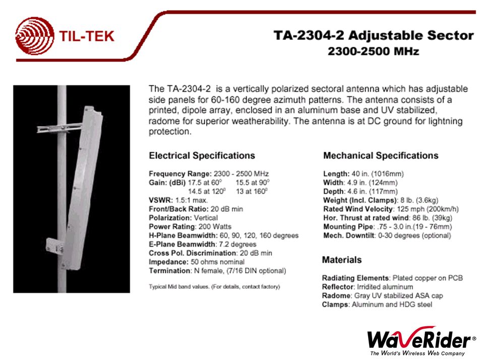
43. Sectoral
directional in nature, but can be adjusted anywhere from 450 to 1800
typical gains vary from 10 to 19 dBi

44. Typical Radiation Pattern for a Sector

45. Omni used at the CCU or Master NCL for wide coverage
typical gains of 3 to 10 dBi

46. Typical Radiation Pattern for an Omni

47. Antenna Radiation Patterns
Common parameters
main lobe (boresight)
half-power beamwidth (HPBW)
front-back ratio (F/B)
pattern nulls
Typically measured in two planes:
Vector electric field referred to E-field
Vector magnetic field referred to H-field

48. Polarization
An antennas polarization is relative to the E-field of antenna.
If the E-field is horizontal, than the antenna is Horizontally Polarized.
If the E-field is vertical, than the antenna is Vertically Polarized.
No matter what polarity you choose, all antennas in the same RF network must be polarized identically regardless of the antenna type.

49. Polarization may deliberately be used to:
Increase isolation from unwanted signal sources (Cross Polarization Discrimination (x-pol) typically 25 dB)
Reduce interference
Help define a specific coverage area
Horizontal
Vertical

50. Antenna Impedance
A proper Impedance Match is essential for maximum power transfer. The antenna must also function as a matching load for the Transmitter ( 50 ohms).
Voltage Standing Wave Ratio (VSWR), is an indicator of how well an antenna matches the transmission line that feeds it.
It is the ratio of the forward voltage to the reflected voltage. The better the match, the Lower the VSWR. A value of 1.5:1 over the frequency band of interest is a practical maximum limit.

51. Return Loss is related to VSWR, and is a measure of the signal power reflected by the antenna relative to the forward power delivered to the antenna.
The higher the value (usually expressed in dB), the better. A figure of 13.9dB is equivalent to a VSWR of 1.5:1. A Return Loss of 20dB is considered quite good, and is equivalent to a VSWR of 1.2:1.

54. Environmental Effects
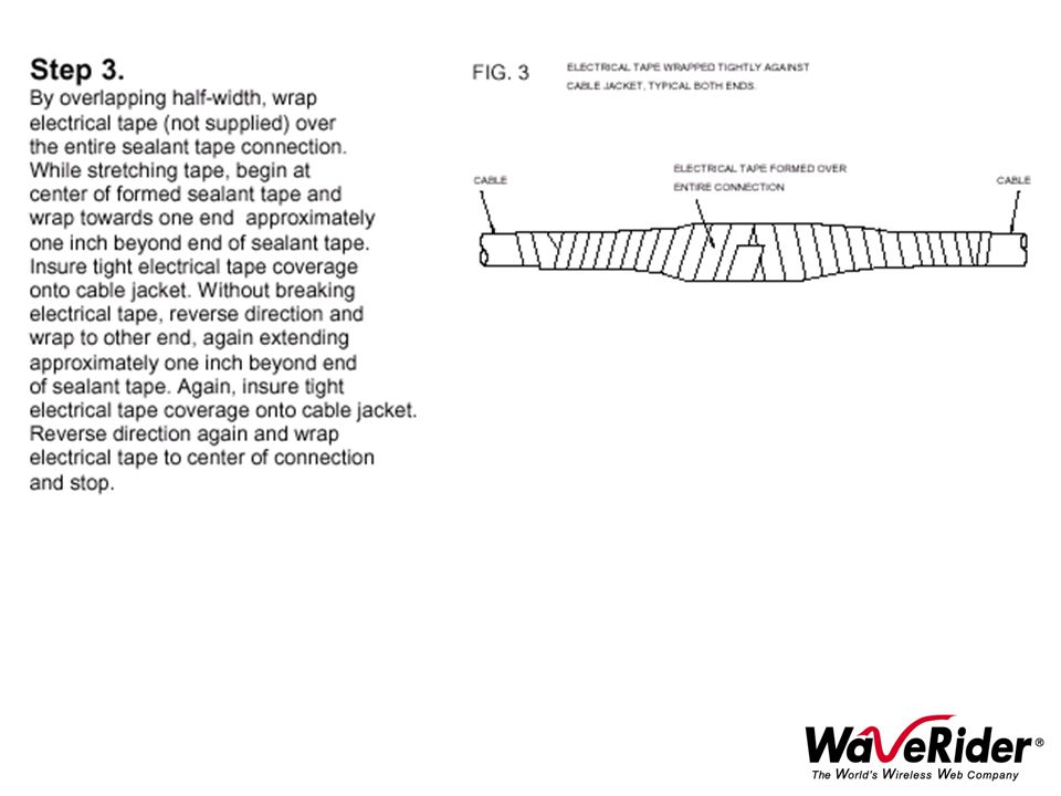
Ice and wind loading, Salt spray
Radomes used to improve performance in icy, windy conditions (more common with larger solid parabolic dishes). Wind loading can be reduced substantially by using a radome.
Wind loading can produce vibration, which in turn can produce azimuth errors. For longer paths, this can be critical.
Installation - pay close attention to proper sealing of all connector junctions.

62. The Transmission Line
The type of cable selected depends mostly on the length of that cable required. Generally, the longer the cable run the better the cable must be in terms of attenuation.
Attenuation refers to the degradation of the signal as it travels through the cable. This is usually stated as a loss in dB per 100 feet.
Andrew Corporation Heliax
Times Microwave
LMR types

63. Attenuation Table

64. Transmission Line Selection
Physical Characteristics:
Bend radius
Diameter - transition considerations (interface ‘jumper cable’ use)
Environmental considerations
Plenum installation (fire retardant)
Special weather-resistant types
UV resistance very important in tropics

65. Line Loss or Attenuation paramount – refer to your Link Budget Calculations to determine how much loss is acceptable and still have a viable link.
Foam dielectric, Air Dielectric, Pressurized types of Coaxial Cable. Waveguide use also possible but typically not cost-effective

66. Connectors
Your connector selection will be determined based on the following:
connector gender at antenna
type of cable being used
use of lightning protection
gender of jumpers being used

67. Antennas – usually Female Lightning Arrestors – usually Female
For the most part the cabling manufacturers also manufacture the connectors that go on the cables. ‘Knock off’ connectors are available, but don’t always fit the cable the way the manufacturers connectors do.
Generally the only decision that needs to be made is what gender of connector to install…Male or Female
Antennas – usually Female
Lightning Arrestors – usually Female

68. Connectors
N-male
RP-SMA- male
N-female
RP-SMA-female

69. The Lightning Arrestor
To avoid the potential for damage during a lightning strike, the use of lightning is highly recommended.
For maximum protection, ground must be connected close to point of entry into building - within 2ft.
Typically structural steel OK for ground connection
Do not use Gas Lines or Water pipes.
Check Electrical Code for grounding restrictions.
Typical Lightning Arrestor

70. Network Feasibility Assessment
Through WaveRiders Professional Services Group (PSG), a Network Feasibility Assessment can be done to establish the viability of a proposed wireless network with either the NCL or LMS products.
System and Program Planning
Implementation Management
Application engineering
Network engineering
Backhaul Design

71. - Electrical Inspection
Certified electrician, equipment grounding
Primary Power Sources
Site Lease / Costs
Antenna
Floor space

72. Link Budget Calculations
To establish the viability of a link prior to installing any equipment, a Link Budget Calculation needs to be made. Performing this calculation will give you an idea as to how much room for path loss you have, and give you an idea as to link quality.
Using the WaveRider Link Path Analysis Tool (LPA Tool), the Fade Margin and other link criteria can be mathematically calculated to determine link quality.

73. Fade Margin
Defined as the difference between the Receive Signal Level RSL, and the Rx Threshold or other chosen reference Level.
For path lengths of 16km or less, a minimum 10dB Fade Margin is recommended
Ie. If you have an RSL of –60dB and a Rx Threshold of –72dB, than your fade Margin would be 12dB

74. Path Loss (dB)
Field Factor (dB)
Antenna Gain
(dBi)
Cable Losses
(dB)
Connector
Losses A B
Received Signal Level
(dBm) = Tx Output (dBm) - Path
Loss(dB) - Field Factor (dB) + Total Antenna Gains (dB) - Total
Cable Losses (dB) - Total Connector Losses (dB)
Tx Output (dBm)

77. Interference Countermeasures
1. Short Paths
2. Narrow Beam Antennas (high gain)
3. Frequency Selection
4. Antenna Polarization
5. Antenna Azimuth
6. Equipment/Antenna Location