Download presentation
Presentation is loading. Please wait.

1
CSE 5808 Quality of Service in Digital Communication Networks
Dr Carlo Kopp, MIEEE, PEng 2005 Semester 1 SCSSE Monash University, Clayton

2
1.1 Introduction Quality of service (QoS) in modern communication networks is about the allocation of network resources to cater for prioritised services. QoS or QOS was used in the Open System Interconnection (OSI) model to indicate the network’s capability to support user’s application in the following categories: Bandwidth: measured in bits, cells or packets per second. Transfer delay: measured by round-trip-time (RTT) Delay jitter or variation: difference in delay impacts on the usage of buffer Traffic loss: measured by cell or packet loss ratio. It is important to certain types of traffic.
 in modern communication networks is about the allocation of network resources to cater for prioritised services. QoS or QOS was used in the Open System Interconnection (OSI) model to indicate the network’s capability to support user’s application in the following categories: Bandwidth: measured in bits, cells or packets per second. Transfer delay: measured by round-trip-time (RTT) Delay jitter or variation: difference in delay impacts on the usage of buffer. Traffic loss: measured by cell or packet loss ratio. It is important to certain types of traffic.")
3
QoS is not just a bandwidth issue.
Since the inception of ISDN, the focus of QoS issues is always on the efficient use of network resources to provide satisfactory qualities to a variety of mission-critical or QoS sensitive services. QoS is not just a bandwidth issue. Bandwidth cannot be increased without a limit for end users. (though technologies such as DWDM can exponentially increase the core or even the complete wired network bandwidth) Bandwidth does not come cheap. Momentary burst of traffic always exists (due to broadcast storms, routing updates, etc.) Application rate Transmission rate
 Bandwidth does not come cheap. Momentary burst of traffic always exists (due to broadcast storms, routing updates, etc.) Application rate. Transmission rate.")
4
QoS study provides a way to prioritize service classes according to their quality needs. Due to the existence of different service classes in modern networks, the concept of sufficient bandwidth becomes even more difficult to judge. Network operators also want to provide “tiered” levels of service. 1.2 A Brief History QoS issues in circuit switched networks are mostly limited to layer 1 (physical), typical parameters are bandwidth, S/N ratio, distortion, attenuation, etc. They have been studied for a long time and most of the problems have been successfully addressed. QoS in modern packet switched networks are dealt with in higher layers of the OSI model (2-7). The typical parameters of concern becomes transfer delay, delay jitter (variation), packet (cell) loss ratio, etc.
, typical parameters are bandwidth, S/N ratio, distortion, attenuation, etc. They have been studied for a long time and most of the problems have been successfully addressed. QoS in modern packet switched networks are dealt with in higher layers of the OSI model (2-7). The typical parameters of concern becomes transfer delay, delay jitter (variation), packet (cell) loss ratio, etc.")
5
1.3 Link, Network and User Level QoS
Facilities regarding to the classification and prioritisation of traffic flow started in X.25 and frame relay networks. X.25 is a protocol suite for earlier, low speed packet switch networks. X.25 packets have header fields for the negotiation of network resource. It has facility to provide connection oriented virtual circuit and special types of packets for flow control. Frame relay provides more bandwidth than X.25. The header has two congestion notification bits, FECN and BECN, which stand for forward and backward explicit congestion notification respectively. The concept of explicit congestion notification is continued in ATM networks and the mechanism to handle congestion is also expanded. IP was initially designed to provide unreliable data transfer. QoS issues were considered by other protocols. This starts to change now. 1.3 Link, Network and User Level QoS Link and network level QoS are technical parameters that can be achieved with appropriate technology.

6
The complete scopes of QoS service are normally defined by end-to- end QoS to customers, i.e from an ingress point to egress point(s). Examples are from A to B or to BCDE. Each QoS domain may be a different service provider using different network technology. B User QoS Region QoS Domain C A QoS Domain User User QoS Domain D E User

7
Examples of service requirement for interactive voice (telephony):
Qualitative and quantitative service levels: qualitative is always relevant to a particular level of service. Examples of service requirement for interactive voice (telephony): Delay ~ 500ms Loss ~ 10-3 Jitter ~ 150ms For MPEG 2 video broadcast: Delay ~ 1000ms Loss ~ Jitter ~ 1ms RTT=40ms, Loss=10-5 Jitter=2ms B User QoS Region QoS Domain C A QoS Domain User User QoS Domain D RTT=low, Loss=medium Jitter=low E User
: Delay ~ 500ms Loss ~ 10-3 Jitter ~ 150ms. For MPEG 2 video broadcast: Delay ~ 1000ms Loss ~ 10-6 Jitter ~ 1ms. RTT=40ms, Loss=10-5 Jitter=2ms. B. User. QoS Region. QoS Domain. C. A. QoS Domain. User. User. QoS Domain. D. RTT=low, Loss=medium Jitter=low. E. User.")
8
1.4 Service Level Agreements (SLAs)
An SLA is mainly a QoS contract between the customer and the service provider. The monitoring of SLAs makes it possible for QoS to be a factor in service charges. Network charges are commonly based on consumption time, volume of traffic, are now also possible on QoS with SLA monitors. SLA monitor is located at service customer/provider boundary. SLA may include the following items: Performance parameters and constraints on the entrance (ingress) and exit (egress) points. Traffic profiles which must be obeyed for the requested service, and disposition of traffic submitted in excess of the profile. Tagging and shaping services for the measurement and conformance of SLA.
 and exit (egress) points. Traffic profiles which must be obeyed for the requested service, and disposition of traffic submitted in excess of the profile. Tagging and shaping services for the measurement and conformance of SLA.")
9
Availability and reliability, failure recovering and rerouting.
Authentication and encryption services. Monitoring and auditing services. Pricing and billing. Examples of SLA (from the reference book of U Black) CIR : Committed Information Rate (as guaranteed rate) PVC: Permanent Virtual Connection
 CIR : Committed Information Rate (as guaranteed rate) PVC: Permanent Virtual Connection.")
10
The overall look of SLA in the QoS hierarchy:
Extra SLA monitoring points can be set up at source/destination end systems, or some other points in the network. The overall look of SLA in the QoS hierarchy: SLA/Traffic contract via UNI/NNI/PNNI Traffic Management Congestion control Buffer control UPC, CAC Flow control, Traffic shaping

11
2.1 Introduction This chapter discusses basic concepts covering QoS control used in packet switched networks. These include traffic credits, congestion notification, packet acknowledgments, flow control, etc. It is common that statistical multiplexing is applied to packet switched networks. This means bandwidth allocation to a source is dynamic according to the momentary amount of traffic flow. Due to traffic fluctuation and the difficulty in knowing precisely the amount of traffic at any given time (multimedia sources, bursty sources, etc.), congestion problems may result, and QoS can be compromised. Network throughput also drops down when congestion occurs.
, congestion problems may result, and QoS can be compromised. Network throughput also drops down when congestion occurs.")
12
2.2 Congestion Control, Connection Admission Control and Usage Parameter Control
Congestion is a condition which exists in link switching nodes or routers, when they are unable to achieve the stated performance objective, which is essential in terms of a QoS guarantee. This diagram is from U Black’s book.

13
Congestion control is used to prevent congestion collapse in the network, this is done through a set of mechanisms and algorithms generally referred to as traffic control. The term congestion control is also used sometimes to refer to some traffic control algorithms, hop by hop or end to end. This can be preventive or reactive, such as ATM-ABR congestion control. Connection Admission Control (CAC) is used by the network to either grant or deny a connection based on the source traffic characteristics, either stated in the SLA, or obtained in some other different ways. The main function of CAC is to ensure that the network is not overloaded with excessive connections which might impair the QoS of existing and incoming connections. Usage Parameter Control (UPC) exists to ensure that admitted connections keep within negotiated constraints and do not violate them either inadvertently or intentionally.
 is used by the network to either grant or deny a connection based on the source traffic characteristics, either stated in the SLA, or obtained in some other different ways. The main function of CAC is to ensure that the network is not overloaded with excessive connections which might impair the QoS of existing and incoming connections. Usage Parameter Control (UPC) exists to ensure that admitted connections keep within negotiated constraints and do not violate them either inadvertently or intentionally.")
14
2.3 Flow Control and Traffic Shaping
Both CAC and UPC reside on the network side as preventive measures intended to avoid network congestion. 2.3 Flow Control and Traffic Shaping These are congestion prevention measures taken at customer sites, although feedback from the network makes them function more effectively. Flow control is used to adjust the source injection rate of traffic into the network. Alternatives are open loop and closed loop control.

15
Open loop control; this is based on an SLA contract
Open loop control; this is based on an SLA contract. Traffic is monitored with possible packet/cell tagging/discarding actions if problems arise. Open loop control is suitable when an SLA exists, the user adheres to the contract and source traffic is predictable. Closed loop control uses a feedback mechanism to direct the source on its emission rate. The feedback messages come from the destination and/or the networks nodes. Closed loop control is suitable when an SLA may or may not exist and traffic may or may not be predictable. The user agrees to accept feedback messages. There two main categories of closed loop flow control, implicit and explicit flow control. Implicit flow control notifies the source the fact that the network is congested or the source is violating its SLA. The source must act according to a predefined function or other relevant policy to reduce the risk of its traffic being tagged or discarded.

16
Explicit flow control contains more information in its feedback message. It normally suggests to the source an explicit rate it should transmit. Explicit rate feedback can happen whether the network is congested or not. It is supposed to advise the source to transmit at a rate best suited to the network situation at the given time. Explicit rate feedback achieves better network throughput when the congestion periods are a lot longer than the end-to-end round trip time (RTT).
.")
17
2.4 Queue Operation and Buffer Size
Explicit rate control requires more network resource than implicit flow control. Traffic shaping is used to smooth out sources so the injection of traffic into the network is more even and predictable. Shaping to real-time traffic must be careful so it does not affect the traffic integrity. Flow control and traffic shaping can be both preventive or reactive. 2.4 Queue Operation and Buffer Size A variety of traffic from different sources is mixed (multiplexed) at the switches and directed to their respective destinations.
 at the switches and directed to their respective destinations.")
18
A switch may consist of many queues as illustrated below:
Conceptually a queue consists of a buffer and a server. The server normally empties the buffer at a constant speed (determined by the output link rate). Given a fixed output link rate, the amount of input traffic, its statistical distribution and size of buffer will direct impact on the QoS. The interval between input packets and their statistical distribution are important indications of the properties of incoming traffic. This is also referred to as packet inter-arrival time.
. Given a fixed output link rate, the amount of input traffic, its statistical distribution and size of buffer will direct impact on the QoS. The interval between input packets and their statistical distribution are important indications of the properties of incoming traffic. This is also referred to as packet inter-arrival time.")
19
The assumption that the process is Poisson may or may not hold.
In order to simplify the study, it is often assumed that the inter-arrival time conforms to Poisson process. An example Poisson probability density function (pdf) is illustrated as follows: The assumption that the process is Poisson may or may not hold. Diagram from U Black’s book
 is illustrated as follows: The assumption that the process is Poisson may or may not hold. Diagram from U Black’s book.")
20
The size of packets is another important indication of the amount of incoming traffic. The size can be variable (X.25, frame relay) or fixed (ATM). Mathematical abbreviations of queues with a single server are: Poisson inter arrival time and fixed packet size: M/D/1 queue Poisson inter arrival time and Poisson packet size: M/M/1 queue Unknown inter arrival time and packet size distribution: G/G/1 queue If the average input traffic amount is fixed, for M/D/1 queue, the cell loss probability decreases linearly with the increase of buffer size. Buffer size is not critical for delay and delay variation if the input traffic load is under 80% (conditions apply). Its effects are clear if the traffic load is over 80%. Larger buffers have bigger delay and jitter. Generally speaking, real-time services require smaller buffers than best effort services. An example buffer size is illustrated on the next page. The sizes of B1=128 cells, B2=300 cells and B3=700 cells.
. Its effects are clear if the traffic load is over 80%. Larger buffers have bigger delay and jitter. Generally speaking, real-time services require smaller buffers than best effort services. An example buffer size is illustrated on the next page. The sizes of B1=128 cells, B2=300 cells and B3=700 cells.")
21
2.5 queueing and Queue Scheduling/Servicing
This is an important measure for QoS maintenance. There are two categories - per class and per VC queueing. Per class queueing groups traffic flows with the same/similar QoS requirements to the same queue. This can be done through the identification of certain VC/VP numbers, or other alternative means. Per VC queueing arranges a queue (or virtual queue) for each VC. This means each VC may have its own QoS priority. B1=128 B2=300 B3=700
 for each VC. This means each VC may have its own QoS priority. B1=128. B2=300. B3=700.")
22
Queue service cycles can be calculated based on the most delay sensitive traffic class. Also queues can be served unevenly, which means some queues are emptied ahead of others.

23
There are two basic types of serving algorithms:
Exhaustive Round Robin (ERR), for the highest-priority queue. The cells are cleared in the highest-priority queue before proceeding to the next highest-priority queue. Queue length-weighted round robin algorithm (QLW RR), for traffic queues which are not extremely delay sensitive. The servicing is based on the type of traffic and the number of cells in the queue. The two algorithms can also be mixed, for example: ERR ERR QLW RR
, for the highest-priority queue. The cells are cleared in the highest-priority queue before proceeding to the next highest-priority queue. Queue length-weighted round robin algorithm (QLW RR), for traffic queues which are not extremely delay sensitive. The servicing is based on the type of traffic and the number of cells in the queue. The two algorithms can also be mixed, for example: ERR. ERR. QLW RR.")
24
2.6 Traffic Tagging and QoS Labeling
A lot of research effort has been devoted on the development of fair and efficient queue length weighted algorithms to improve QoS. The example on the next page (U Black) shows the transmission of two compressed voice channels sharing a 64kbit/s bandwidth with a TCP file transfer application. The improvement is clear. 2.6 Traffic Tagging and QoS Labeling Traffic tagging happens at the ingress point of the user into network interface (UNI) . A QoS function such as UPC (Usage Parameter Control), or CAC (Connection Admission Control) is used. This happens if the user is violating its SLA (UPC), or the provider’s network is very congested (CAC to deny connection or tag traffic?). The tagged traffic packets receive a lower QoS guarantee. They are likely to be discarded first in the event of congestion arising.
 shows the transmission of two compressed voice channels sharing a 64kbit/s bandwidth with a TCP file transfer application. The improvement is clear. 2.6 Traffic Tagging and QoS Labeling. Traffic tagging happens at the ingress point of the user into network interface (UNI) . A QoS function such as UPC (Usage Parameter Control), or CAC (Connection Admission Control) is used. This happens if the user is violating its SLA (UPC), or the provider’s network is very congested (CAC to deny connection or tag traffic ). The tagged traffic packets receive a lower QoS guarantee. They are likely to be discarded first in the event of congestion arising.")
26
Labels are often used as QoS indicators in the header of a packet.
Label values can be fixed at the source and used thereafter to identify the packet in terms of QoS and other parameters. More often, the values are changed at each switching node, which is referred to as label swapping, mapping or marking. A mapping table is normally used to associate incoming packet labels and their QoS implications with outgoing ones. BT: burst tolerance. PDV: packet delay variation

27
2.7 Window Based Flow Control
Also referred to as sliding window flow control. The idea is to tune the size of window so the network bandwidth is fully occupied but no congestion is caused. The transmitter and receiver have the same (virtual) window placed on the transmission/reception data stream. There are three important parameters for a window: Lower Edge Pointer (LEP), marks the position of window in the data stream. Progress Pointer (PP), marks the transmission or reception progress in the window. Window Size (WS), marks the coverage of the window in the data stream. The initial window size may be determined by the size of receiver buffer or some other factors.
 window placed on the transmission/reception data stream. There are three important parameters for a window: Lower Edge Pointer (LEP), marks the position of window in the data stream. Progress Pointer (PP), marks the transmission or reception progress in the window. Window Size (WS), marks the coverage of the window in the data stream. The initial window size may be determined by the size of receiver buffer or some other factors.")
28
Any data to the left of LEP has been sent and acknowledged.
The operation is based on a transmission/acknowledgement (TR/ACK) mechanism. Any data to the left of LEP has been sent and acknowledged. Data between LEP and PP has been sent but not acknowledged. Data to the right of PP has not been sent, and the PP cannot proceed beyond the upper edge (LEP+WS). LEP can move forward in two ways, a) when the ACK of data packet immediately next to it arrives, or b) all ACKs in the window arrive. If WS=1, the mechanism becomes simple TR/ACK. WS and timeout, retransmission are issues under research. … … LEP PP The window
 mechanism. Any data to the left of LEP has been sent and acknowledged. Data between LEP and PP has been sent but not acknowledged. Data to the right of PP has not been sent, and the PP cannot proceed beyond the upper edge (LEP+WS). LEP can move forward in two ways, a) when the ACK of data packet immediately next to it arrives, or b) all ACKs in the window arrive. If WS=1, the mechanism becomes simple TR/ACK. WS and timeout, retransmission are issues under research … … LEP. PP. The window.")
29
3.1 Introduction 3.2 Network Interfaces
This chapter introduces more general ideas about network QoS operations. These include QoS reference points, connection types, switching and routing principles for QoS maintenance. 3.2 Network Interfaces These are used as QoS reference points. Protocol standards exist to define the User to Network Interface (UNI), Network to Network interface (PNNI, AINI) and other relevant interfaces. Certain network technologies such as IP were originally designed for inter-networking and have no specifications on interfaces. QoS sensitive services are changing the situation (eg. VoIP).
, Network to Network interface (PNNI, AINI) and other relevant interfaces. Certain network technologies such as IP were originally designed for inter-networking and have no specifications on interfaces. QoS sensitive services are changing the situation (eg. VoIP).")
30
Connection-oriented and connectionless interfaces:
Connection oriented: connection establishmentdata transfer connection release. A connection is usually mapped out with fixed routes in network. QoS provision is inherent. Connectionless: no connection is established for data transfer. Each individual packet carries the full address for destination. QoS provisions are emerging. 3.2 Layered QoS Model The network does not necessarily need to be aware of the user QoS requirement at the physical and link layers. Resources at these layers are allocated according to QoS information set up in higher layers. QoS provisioning information is passed hop by hop from source to destination to set up all switches en route.

32
3.3 Switching and Routing Technologies
Circuit switching: the source and the destination are given a “wired” connection, or fixed time slots. Traditional telephone switching system. The delay and jitter are constant. Other services can be built on this type of connection to improve efficiency. TDM: Time division multiplexing TSI: Time Slot Interexchange

33
Message switching: this is a store-and-forward technology
Message switching: this is a store-and-forward technology. The messages are collected and stored temporarily on disk units at the switches and then forwarded according to the header message. It was used between the 60s and the 70s. Packet switching: user data are divided into smaller pieces (packets), each with complete protocol control information (headers). The smaller pieces are easier to handle at switches. The topology of networks also allows alternative routes should one connection becomes congested or faculty. This is contemporary switching technology.
, each with complete protocol control information (headers). The smaller pieces are easier to handle at switches. The topology of networks also allows alternative routes should one connection becomes congested or faculty. This is contemporary switching technology.")
34
Technologies that we are interested in supporting involve packet switching (with certain QoS level considerations), X.25 (not really used any more), Frame Relay (still in use to some extent), ATM (most commonly used technology currently), and IP (a higher layer for DTE address portability).
, X.25 (not really used any more), Frame Relay (still in use to some extent), ATM (most commonly used technology currently), and IP (a higher layer for DTE address portability).")
35
3.4 A Brief Technology Overview
The following table is from U Black’s book.

37
3.5 Effective Use of a Packet Header
Switching/routing information contained in the headers (labels) are the key to fast forwarding and thus important for QoS.
 are the key to fast forwarding and thus important for QoS.")
38
4.1 Introduction ATM technology provides the most comprehensive QoS facilities to date. Fixed size packets – called cells - are the basic transfer units. These consist of 48 bytes of payload and 5 bytes of header.

39
GFC is a 4-bit field that provides a framework for flow control and fairness to the access segment (a). The GFC field is not used in the network segment (b). VPI/VCI: virtual path/connection identifiers. PT: payload type, for example, user cell, signaling, or OAM cell. CLP: single bit cell loss priority (0 means higher priority and 1 lower priority, discard first), and HEC is header error check. Applications generally access the ATM transport layer via an ATM adaptation layer (AAL) (ITU-T I.363). Eg. AAL1 is for CBR traffic requiring synchronisation, or circuit emulation. AAL2 was proposed for VBR but new functions have been added to it, and AAL5 is for data service (also used for video to gain efficiency). ATM network has traffic management definitions (ITU-T I.371, ATM Forum TM4.0) mostly for QoS provision and guarantee. Signaling and routing (UNI, PNNI, AINI, etc) are also used to facilitate the provision of QoS.
, and HEC is header error check. Applications generally access the ATM transport layer via an ATM adaptation layer (AAL) (ITU-T I.363). Eg. AAL1 is for CBR traffic requiring synchronisation, or circuit emulation. AAL2 was proposed for VBR but new functions have been added to it, and AAL5 is for data service (also used for video to gain efficiency). ATM network has traffic management definitions (ITU-T I.371, ATM Forum TM4.0) mostly for QoS provision and guarantee. Signaling and routing (UNI, PNNI, AINI, etc) are also used to facilitate the provision of QoS.")
40
4.2 ATM Traffic Classes and QoS Demands

41
CBR is constant bit rate service
CBR is constant bit rate service. The traffic is described by a PCR (peak cell rate). It has clear goals in terms of CLR (cell loss ratio), Max-CTD (maximum cell transfer delay) and P2P-CDV (peak to peak cell delay variation). PCR represents the peak emission rate of the source. The inverse of the PCR represents the minimum inter-arrival time of cells. PCR can be limited by the physical link speed of the source or via shaping the ingress traffic. (following diagram from N. Giroux) Real-time VBR (variable bit rate). The traffic is described by PCR, SCR (sustained cell rate) and MBS (maximum burst size). SCR is an upper bound on the average transmission rate over time scales that are relatively long to those for which the PCR is defined.
. It has clear goals in terms of CLR (cell loss ratio), Max-CTD (maximum cell transfer delay) and P2P-CDV (peak to peak cell delay variation). PCR represents the peak emission rate of the source. The inverse of the PCR represents the minimum inter-arrival time of cells. PCR can be limited by the physical link speed of the source or via shaping the ingress traffic. (following diagram from N. Giroux) Real-time VBR (variable bit rate). The traffic is described by PCR, SCR (sustained cell rate) and MBS (maximum burst size). SCR is an upper bound on the average transmission rate over time scales that are relatively long to those for which the PCR is defined.")
42
The SCR is always specified along with a corresponding MBS.
The MBS parameter represents the burstiness factor. It specifies the maximum number of cells that can be transmitted at PCR while complying with the negotiated SCR. SCR can be defined for the aggregate of all cell flows, or only for the higher priority cells (CLP=0). In the latter case, cells with a CLP=1 can exceed the SCR, and up to PCR.
. In the latter case, cells with a CLP=1 can exceed the SCR, and up to PCR.")
43
The difference between RT VBR and NRT VBR is that RT VBR requires all of CLR, Max-CTD and P2P-CDV, while NRT VBR only requires CLR. The ABR (available bit rate) service can guarantee a minimum of bandwidth. The transmission rate may be higher if bandwidth is available. The source participates in a well defined feedback flow control mechanism together with network switches and destination. ABR is an important congestion control measure in ATM networks, but may be expensive to implement. Conforming ABR traffic should experience minimum cell loss in the network, although CLR is not explicitly required. The GFR (guaranteed frame rate) guarantees a minimum amount of bandwidth. CLR is kept to a minimum if the traffic rate is within this limit. No QoS guarantee if the traffic rate exceeds the limit. The GFR does not need to conform to any flow control mechanism. The GFR service is designed to deal with protocol data units (PDU) from the layer above AAL (eg. TCP/IP).
 service can guarantee a minimum of bandwidth. The transmission rate may be higher if bandwidth is available. The source participates in a well defined feedback flow control mechanism together with network switches and destination. ABR is an important congestion control measure in ATM networks, but may be expensive to implement. Conforming ABR traffic should experience minimum cell loss in the network, although CLR is not explicitly required. The GFR (guaranteed frame rate) guarantees a minimum amount of bandwidth. CLR is kept to a minimum if the traffic rate is within this limit. No QoS guarantee if the traffic rate exceeds the limit. The GFR does not need to conform to any flow control mechanism. The GFR service is designed to deal with protocol data units (PDU) from the layer above AAL (eg. TCP/IP).")
44
4.3 Definition of Major QoS Parameters
The network aims to discard complete PDUs instead of dropping cells randomly under congestion. MCR (minimum cell rate) stands for the minimum allocated bandwidth for a connection. MFS is the maximum frame size which defines the maximum size of an AAL protocol data unit that can be sent on a GFR connection. 4.3 Definition of Major QoS Parameters There are three negotiable parameters between the end systems and the network: CLR: cell loss ratio Max-CTD: maximum cell transfer delay P2P-CDV: peak-to-peak cell delay variation There are three non negotiable parameters: CER: cell error ratio
 stands for the minimum allocated bandwidth for a connection. MFS is the maximum frame size which defines the maximum size of an AAL protocol data unit that can be sent on a GFR connection. 4.3 Definition of Major QoS Parameters. There are three negotiable parameters between the end systems and the network: CLR: cell loss ratio. Max-CTD: maximum cell transfer delay. P2P-CDV: peak-to-peak cell delay variation. There are three non negotiable parameters: CER: cell error ratio.")
45
SECBR: severely errored cell block ratio
CMR: cell misinsertion rate CLR is defined as Lost Cells/Total Transmitted Cells. Total Transmitted Cells counts only the conforming cells. A cell is lost if any of the following happens: It never reached its destination It was received with an invalid header Its contents were corrupted by errors Cell Transfer Delay generally consists of two parts: queueing delay and propagation delay. The former is in switches and latter with transmission line (about 5us per km with optical fibre). The minimum transfer delay would be propagation delay only. The CTD for each cell is normally different depending on queueing and queue scheduling algorithms.
. The minimum transfer delay would be propagation delay only. The CTD for each cell is normally different depending on queueing and queue scheduling algorithms.")
46
The maximum cell transfer delay (Max-CTD) represents the (1-) quantile of the CTD probability density function. The selection of can be network specific which will create the statistical distribution of CTD. It is safe to select CLR as .. P2P-CDV represents the difference between the maximum CTD and the minimum CTD, this is the Max-CTD minus the fixed delay.

47
4.4 Measurement of Delay Parameters
The cell error ratio (CER) is defined as Errored cells/(Successfully transferred cells + Errored cells). An errored cell is a cell that has had some of its content (header or payload) modified erroneously and cannot be recovered. Severely errored cell block ratio (SECBR) = Severely errored cell blocks/Total transmitted cell blocks. A cell block is a sequence of N cells transmitted consecutively on a given connection. Practically, this can be user information cells transmitted between successive OAM cells. Cell misinsertion rate (CMR) = Misinserted cells/Time interval. A misinserted cell is a cell that is carried over a VC to which it does not belong. This is most likely due to an undetected error in the header. 4.4 Measurement of Delay Parameters This section discusses some aspects of ITU-T I.356, which is about ATM layer cell transfer performance.
 is defined as Errored cells/(Successfully transferred cells + Errored cells). An errored cell is a cell that has had some of its content (header or payload) modified erroneously and cannot be recovered. Severely errored cell block ratio (SECBR) = Severely errored cell blocks/Total transmitted cell blocks. A cell block is a sequence of N cells transmitted consecutively on a given connection. Practically, this can be user information cells transmitted between successive OAM cells. Cell misinsertion rate (CMR) = Misinserted cells/Time interval. A misinserted cell is a cell that is carried over a VC to which it does not belong. This is most likely due to an undetected error in the header. 4.4 Measurement of Delay Parameters. This section discusses some aspects of ITU-T I.356, which is about ATM layer cell transfer performance.")
48
One-Point CDV: This describes the variability in the pattern of cell arrivals with reference to the PCR. It measures cell clumping and gaps. The one-point CDV of a cell, k is defined as: Where, Rik is the reference arrival time, and Aik is the actual arrival time. To start with, Ri1=Ai1. The reference time is calculated based on the previous cell arrival and PCR, as follows: The above equation indicates that if there is a large gap in cell arrivals, then the actual arrival time will be used to produce the next reference arrival time, otherwise, the previous reference arrival time will be used. We assume k 2 in the above equation. If Ri(k-1) Ai(k-1) otherwise
 Ai(k-1) otherwise.")
49
The diagram should be read from right to left, we have:
For example: A source is transmitting at the PCR of one cell for every 4 slots with a one slot fixed transmission delay. The arrival pattern is illustrated as follows: The diagram should be read from right to left, we have: Ai1=2, Ri1=2, CDVi1=0, and Ri2=Ai1+4=6 Ai2=11, Ri2=6, CDVi2=-5, and Ri3=Ai2+4=15 Ai3=12, Ri3=15, CDVi3=3, and Ri4=Ri3+4=19 Ai4=14, Ri4=19, CDVi4=5, and Ri5= Ri4+4=23 Ai5=18, Ri5=23, CDVi5=5, and Ri6= Ri5+4=27 Ai6=22, Ri6=27, CDVi6=5, and Ri7= Ri6+4=31 Ai7=26, Ri7=31, CDVi7=5, and Ri8= Ri7+4=35 2 11

50
Two-Point CDV: This represents the cell arrival pattern with reference to the cell pattern generated by the source. It is measured between two reference points in the network (e.g. ingress and egress UNI). The two- point CDV can be defined as: Where CTDRk is reference cell delay and CTDAk is actual cell delay. CTDRk is defined as the cell delay experienced by the first cell. For example: CDVj1 =0, CDVj2 =(13-5)-3=5, CDVj3 =(14-9)-3=2, CDVj4 =(15-13)- 3=-1, CDVj5 =(20-17)-3=0. 5 1 20 13 4
-3=5, CDVj3 =(14-9)-3=2, CDVj4 =(15-13)- 3=-1, CDVj5 =(20-17)-3=")
51
Negative CDVjk means the cell arrives with a smaller CTD than the first cell, otherwise it has a greater CTD than the first cell. Two-point CDV is often difficult to obtain since user cells do not always have time stamps. The maximum CDV for CBR can be obtained using the one-point CDVik previously. A positive CDVik means the kth cell experienced a smaller delay than the maximum delay experienced up to (k-1)th cell, otherwise, the it is larger than the maximum delay. The definition, CDVk is given in the following equation. It is an approximation of the two point CDV. CDV0 is set to 0 to start with. If CDVik 0 otherwise
th cell, otherwise, the it is larger than the maximum delay. The definition, CDVk is given in the following equation. It is an approximation of the two point CDV. CDV0 is set to 0 to start with. If CDVik 0. otherwise.")
52
With the example we had before, we can re-calculate CDVk.
CDV0=0, CDVi1=0, so CDV1=0 CDV1=0, CDVi2=-5, so CDV2=5 CDV2=5, CDVi3=3, so CDV3=5 CDV3=5, CDVi4=5, so CDV4=5 CDV4=5, CDVi5=5, so CDV5=5 CDV5=5, CDVi6=5, so CDV6=5 CDV6=5, CDVi7=5, so CDV7=5

53
5.1 Introduction This chapter discusses issues related to traffic compliance, traffic- shaping and policing. This is important since resources allocated according to the traffic descriptors may not guarantee the QoS in case they are exceeded (intentionally or inadvertently). Violation of traffic descriptors by individual sources may also impact on the QoS of other well behaving sources. If an application does not “naturally” behave according to the traffic descriptors, the traffic output needs to be “shaped” to ensure compliance. Traffic shaping is a voluntary measure taken by users (not required by standards TM4.0 and I.371) to improve conformance and hence avoid QoS degradation.
. Violation of traffic descriptors by individual sources may also impact on the QoS of other well behaving sources. If an application does not naturally behave according to the traffic descriptors, the traffic output needs to be shaped to ensure compliance. Traffic shaping is a voluntary measure taken by users (not required by standards TM4.0 and I.371) to improve conformance and hence avoid QoS degradation.")
54
To ensure compliances of sources, the network monitors or “polices” on the incoming traffic at the entry point. For a connection, the cell conformance check is carried out by an algorithm called the generic cell rate algorithm (GCRA). GCRA monitors traffic with the set of contracted descriptors, and takes one of the three following actions on a non-conforming cell: Tagging the cell Discarding the cell No action Tagging means degrading a high priority cell (CLP=0) to a low priority cell (CLP=1). The cell does not receive a QoS guarantee, although it may still reach the destination. The traffic monitor can also incorporate a shaping buffer to delay the emission of non-conforming cells. This capability is termed soft policing. The network can also “shape” the source according to the GCRA instead of policing it. This means some more computational cost in switches. Shaping at the source is the ideal option.
. GCRA monitors traffic with the set of contracted descriptors, and takes one of the three following actions on a non-conforming cell: Tagging the cell. Discarding the cell. No action. Tagging means degrading a high priority cell (CLP=0) to a low priority cell (CLP=1). The cell does not receive a QoS guarantee, although it may still reach the destination. The traffic monitor can also incorporate a shaping buffer to delay the emission of non-conforming cells. This capability is termed soft policing. The network can also shape the source according to the GCRA instead of policing it. This means some more computational cost in switches. Shaping at the source is the ideal option.")
55
5.2 The Definition of Conformance
Conformance definitions varie with different classes of traffic. Flexibility also exists within a single class of service. A QoS guarantee is applicable to cells with a CLP=0 in some cases and CLP=0+1 in other situations. This is listed in the following table.

56
For the CBR service, there is only one conformance definition that treats all cells equally, CLP transparent. If PCR for all cells is observed, QoS in terms of CLR, CTD and CDV will be provided. VRB.1 conformance definition is fully CLP transparent. VBR.2 and VBR.3 conformance definitions are more flexible and allow the traffic to exceed the SCR up to PCR. Only cells with CLP=0 need to observe SCR limit, and their QoS will be guaranteed. The difference of VBR.2 and VBR.3 is the action taken on non- conforming cells. VBR.3 tags them while VBR.2 discards them on the assumption that those cells are tagged already. ABR service has one conformance definition. There is no CLP=1 cell for this service category. MCR is not quite a conformance definition but defines the minimum set of cells eligible for QoS regardless of network congestion status. For GFR, conformance applies to PCR only on aggregate traffic. The MCR is again used to define QoS eligibility.

57
5.3 Cell Conformance Analysis
The two GFRs differ again only with the action on non-conforming cells. For UBR service, the conformance is applicable on the PCR for all cells. No QoS is guaranteed even if traffic is conforming. Non- conforming cells may be discarded (UBR.1) or tagged (UBR.2). CLP should be transparent to QoS if different categories or sub- categories are aggregated. 5.3 Cell Conformance Analysis The generic cell rate algorithm (GCRA) can be used to analyse and police cell conformance. It can also be used for conformance shaping. The GCRA is applied differently for various service categories. The essence is a leaky bucket algorithm. 5.3.1 Conformance for the CBR Service In the ideal case, a cell is not conforming if it arrives earlier than 1/PCR.
 or tagged (UBR.2). CLP should be transparent to QoS if different categories or sub- categories are aggregated. 5.3 Cell Conformance Analysis. The generic cell rate algorithm (GCRA) can be used to analyse and police cell conformance. It can also be used for conformance shaping. The GCRA is applied differently for various service categories. The essence is a leaky bucket algorithm Conformance for the CBR Service. In the ideal case, a cell is not conforming if it arrives earlier than 1/PCR.")
58
In practical terms the initial traffic pattern may be jittered with a delay variation due to the multiplexing of connections. To account for jitter, a tolerance factor is introduced. This is referred to as cell delay variation tolerance (CDVT). The GCRA for CBR has two parameters, an increment I=1/PCR and a limit L=CDVT. The GCRA(I, L) is described as follows. The GCRA can be expressed as a leaky bucket algorithm, with the analogy that as a bucket with the capacity of Bq (units), it continuously leaks (decrements) one units each time unit passes. It increments by I=1/PCR units after each conforming cell arrives. Obviously Bq returns to zero prior to the arrival of the next cell if the arrival pattern is evenly spread at I units per cell. Bq has a residual value if the inter arrival time is shorter than I. The bucket (Bq) has an upper limit which is L=CDVT, and a lower limit of 0. At the arrival of a cell, if Bq L, then Bq is incremented by I, and the cell is conforming, if Bq>L, the cell is non-conforming, and Bq is not incremented.
. The GCRA for CBR has two parameters, an increment I=1/PCR and a limit L=CDVT. The GCRA(I, L) is described as follows. The GCRA can be expressed as a leaky bucket algorithm, with the analogy that as a bucket with the capacity of Bq (units), it continuously leaks (decrements) one units each time unit passes. It increments by I=1/PCR units after each conforming cell arrives. Obviously Bq returns to zero prior to the arrival of the next cell if the arrival pattern is evenly spread at I units per cell. Bq has a residual value if the inter arrival time is shorter than I. The bucket (Bq) has an upper limit which is L=CDVT, and a lower limit of 0. At the arrival of a cell, if Bq L, then Bq is incremented by I, and the cell is conforming, if Bq>L, the cell is non-conforming, and Bq is not incremented.")
59
Bq is set to 0 to start with.
Yes No Cell arrives? Bq=max(0, Bq-1) No Bq>L Yes At each time unit Cell conforming Cell non- conforming Bq=Bq+I
 No. Bq>L. Yes. At each time unit. Cell conforming. Cell non- conforming. Bq=Bq+I.")
60
In the standard, a non-decrementing value B is used instead of Bq, and it uses a process ta – LCT to represent the leaking process, illustrated as follows (N. Giroux), where ta is the current cell arrival time, and LCT stands for last conforming cell arrival time. Bq=max[0, B-(ta – LCT)]. The leaky bucket algorithm can be modified slightly to form the virtual scheduling algorithm. If a cell arrives at ta, it is compared with a theoretical (or reference) arrival time (TAT). If ta TAT-L, the cell is conformant, otherwise it is not. B=B
![In the standard, a non-decrementing value B is used instead of Bq, and it uses a process ta – LCT to represent the leaking process, illustrated as follows (N. Giroux), where ta is the current cell arrival time, and LCT stands for last conforming cell arrival time. Bq=max[0, B-(ta – LCT)].](http://slideplayer.com/slide/2436949/8/images/60/In+the+standard%2C+a+non-decrementing+value+B+is+used+instead+of+Bq%2C+and+it+uses+a+process+ta+%E2%80%93+LCT+to+represent+the+leaking+process%2C+illustrated+as+follows+%28N.+Giroux%29%2C+where+ta+is+the+current+cell+arrival+time%2C+and+LCT+stands+for+last+conforming+cell+arrival+time.+Bq%3Dmax%5B0%2C+B-%28ta+%E2%80%93+LCT%29%5D..jpg "The leaky bucket algorithm can be modified slightly to form the virtual scheduling algorithm. If a cell arrives at ta, it is compared with a theoretical (or reference) arrival time (TAT). If ta TAT-L, the cell is conformant, otherwise it is not. B=B.")
61
For example, a CBR (I=4) cell stream as follows was jittered and analyzed by the above discussed algorithms: TAT=TAT

62
If L=2, then we have the following results:
This means that cell number 3 and 5 are marked as non-conforming. If L is 3, which means the requirement is more relaxed. Then only cell 6 is marked as non-conforming. Bq if the negatives are set zero

63
5.3.2 Conformance for the VBR Service
VBR conformance is defined on both the SCR and the PCR. The PCR is always defined on both CLP=1 and 0 traffic. The SCR can be on the aggregate (VBR.1) or on the CLP=0 only (VBR.2 and .3). The SCR is evaluated by the same algorithm as for the PCR.
 or on the CLP=0 only (VBR.2 and .3). The SCR is evaluated by the same algorithm as for the PCR.")
64
The PCR conformance monitoring is the same as in the case of CBR.
For SCR, the increment is set to 1/SCR, and the CDVT is replaced by a value represented by burst tolerance (BT) added to itself. BT is calculated based on PCR and SCR. The limit for SCR is therefore, BT+CDVT. The algorithm of GCRA (Ip, Lp, Is, Ls) is referred to as Dual Leaky Bucket (dual virtual scheduling), where Ip, Lp are for PCR and Is, Ls are for SCR. For VBR.1, a cell must conform both the PCR and SCR to be classified as conforming. For VBR.2 and VBR.3, a CLP=0 cell must conform both PCR and SCR, and CLP=1 cells only need to conform to the PCR.
 added to itself. BT is calculated based on PCR and SCR. The limit for SCR is therefore, BT+CDVT. The algorithm of GCRA (Ip, Lp, Is, Ls) is referred to as Dual Leaky Bucket (dual virtual scheduling), where Ip, Lp are for PCR and Is, Ls are for SCR. For VBR.1, a cell must conform both the PCR and SCR to be classified as conforming. For VBR.2 and VBR.3, a CLP=0 cell must conform both PCR and SCR, and CLP=1 cells only need to conform to the PCR.")
65
Dual leaky bucket algorithm for VBR.1
The situation is slightly more complex for VBR.2 and VBR.3. The algorithm needs to check the status of CLP.

67
The dual virtual scheduling algorithm for VBR.1 is given as follows:
The dual virtual scheduling algorithm for VBR.2 and VBR.3 is given on the next page.

69
For example: ten continuous cells with CLP=0 transmitted at the maximum line speed. Is=4, Ip=2, Ls=7, Lp=1, analyze cell conformance. The results are the same with VBR.1 and VBR.2, as follows: 9 8

70
The result is slightly different for VBR.3, shown as follows:

71
5.3.3 Conformance for ABR, GFR and UBR Services
ABR traffic rate varies with the congestion status of the network. A dynamic GCRA or D-GCRA can be used in the explicit rate mode. This means the rate indicated in the backward resource management (RM) cell will determine the GCRA parameters. In any case, conforming ABR cell rate cannot be more than PCR. Conformance to the GFR service is governed by the following three tests: Conformance to GCRA(1/PCR0+1, CDVTPCR) for the aggregate flow. All cells of the frame have the same CLP value Conformance to the maximum frame size (MFS). A cell conforms to this test if the number of cells from the last frame boundary up to and including this cell is less than MFS.
 cell will determine the GCRA parameters. In any case, conforming ABR cell rate cannot be more than PCR. Conformance to the GFR service is governed by the following three tests: Conformance to GCRA(1/PCR0+1, CDVTPCR) for the aggregate flow. All cells of the frame have the same CLP value. Conformance to the maximum frame size (MFS). A cell conforms to this test if the number of cells from the last frame boundary up to and including this cell is less than MFS.")
72
A frame conforms if all cells in the frame conform
A frame conforms if all cells in the frame conform. If a cell in the frame does not conform, the following actions will be taken: First cell: discard the whole frame Not the first cell: discard it and remaining cells of the frame, except for the last cell to keep frame boundary. The MCR QoS guarantee applies to complete unmarked, conformant frames. A frame based GCRA or F-GCRA can be used for this check. The parameters for F-GCRA are (1/MCR0, BT+CDVTMCR) Frames not eligible for the QoS guarantee may be discarded or tagged, depending on whether it is GFR.1 or GFR.2. In GFR.1, the network is not allowed to tag cells of an unmarked frame ineligible for MCR QoS guarantee. In GFR.2, the network is allowed to tag cells of an unmarked frame but should attempt to tag only complete frames. (If the whole frame is buffered, refer to MFS) The network is not required to perform the MCR/F-GCRA check. MCR QoS can be guaranteed through scheduling of the VC queue.
 Frames not eligible for the QoS guarantee may be discarded or tagged, depending on whether it is GFR.1 or GFR.2. In GFR.1, the network is not allowed to tag cells of an unmarked frame ineligible for MCR QoS guarantee. In GFR.2, the network is allowed to tag cells of an unmarked frame but should attempt to tag only complete frames. (If the whole frame is buffered, refer to MFS) The network is not required to perform the MCR/F-GCRA check. MCR QoS can be guaranteed through scheduling of the VC queue.")
73
5.4 Traffic Policing and Shaping
UBR conformance is defined on the PCR of the aggregate flow, like the CBR. Conforming UBR cells will not be guaranteed for QoS. 5.4 Traffic Policing and Shaping Traffic policing includes usage parameter control or UPC (between the user and network) and network parameter control NPC (between two networks). The policing of traffic in different categories involves conformance checking and discarding non-conforming cells. The purpose of shaping is to produce conformant cell streams. Reverse leaky bucket or reverse virtual-scheduling algorithms can be used. Shaping is also related to queue scheduling, which will be discussed in detail in other chapters. The reverse leaky bucket for CBR/PCR: a cell is transmitted if the bucket (B) is empty.
 and network parameter control NPC (between two networks). The policing of traffic in different categories involves conformance checking and discarding non-conforming cells. The purpose of shaping is to produce conformant cell streams. Reverse leaky bucket or reverse virtual-scheduling algorithms can be used. Shaping is also related to queue scheduling, which will be discussed in detail in other chapters. The reverse leaky bucket for CBR/PCR: a cell is transmitted if the bucket (B) is empty.")
74
When a cell is transmitted, the bucket fills by I=1/PCR units.
Reverse virtual-scheduling for CBR/PCR: a conforming emission time (CET) is kept by a timer. Each time CET is reached, a cell is transmitted, and CET=CET+I, where I=1/PCR. For example, there are 8 consecutive cells in the buffer and I=1/PCR=2, which is half the line speed. It can be seen that the cell release occurs every other time unit.
 is kept by a timer. Each time CET is reached, a cell is transmitted, and CET=CET+I, where I=1/PCR. For example, there are 8 consecutive cells in the buffer and I=1/PCR=2, which is half the line speed. It can be seen that the cell release occurs every other time unit.")
75
For VBR/PCR-SCR, a reverse dual leaky bucket, or reverse dual virtual scheduling is used.
For VBR.1, a cell is scheduled for transmission (regardless of CLP bit), if the PCR bucket (Bp) is empty and SCR bucket (Bs) is lower than BT. When the cell is scheduled to be transmitted, the Bp bucket fills by Ip=1/PCR and Bs bucket by Is =1/SCR units. VBR.2 and VBR.3 can be shaped the same way as the VBR.1. They can also be shaped in a slightly different way. The PCR bucket (Bp) must be empty for VBR.2 or VBR.3 to schedule the transmission of any cell. The CLP=1 cells can be scheduled without the SCR or Bs check. CLP=0 cells can also be transmitted if the SCR check fails by turning the CLP bit into 1. When a CLP=1 cell is scheduled without passing the SCR check, the bucket Bs is not incremented.
, if the PCR bucket (Bp) is empty and SCR bucket (Bs) is lower than BT. When the cell is scheduled to be transmitted, the Bp bucket fills by Ip=1/PCR and Bs bucket by Is =1/SCR units. VBR.2 and VBR.3 can be shaped the same way as the VBR.1. They can also be shaped in a slightly different way. The PCR bucket (Bp) must be empty for VBR.2 or VBR.3 to schedule the transmission of any cell. The CLP=1 cells can be scheduled without the SCR or Bs check. CLP=0 cells can also be transmitted if the SCR check fails by turning the CLP bit into 1. When a CLP=1 cell is scheduled without passing the SCR check, the bucket Bs is not incremented.")
76
Reverse dual scheduling scheme for VBR
Reverse dual scheduling scheme for VBR.1 keeps CETs and CETp for each connection. The conforming emission time (CET) for the connection is CET=max(CETs-BT, CETp). A cell is scheduled to transmit when this value is reached. CETs = ta + Is and CETp = ta +Ip after a cell is transmitted at time ta. VBR.2 and VBR.3 again can be shaped the same way as VBR.1 if the cell cannot be tagged. If a tagging function is available, shaping can be carried out on CETp only. Cells can be transmitted with CLP=1 when CETs-BT>CETp. The following example assumes VBR.1 shaping with Ip=2, Is=4, BT=6, the source is transmitting at the line speed with a CLP=0.
 for the connection is CET=max(CETs-BT, CETp). A cell is scheduled to transmit when this value is reached. CETs = ta + Is and CETp = ta +Ip after a cell is transmitted at time ta. VBR.2 and VBR.3 again can be shaped the same way as VBR.1 if the cell cannot be tagged. If a tagging function is available, shaping can be carried out on CETp only. Cells can be transmitted with CLP=1 when CETs-BT>CETp. The following example assumes VBR.1 shaping with Ip=2, Is=4, BT=6, the source is transmitting at the line speed with a CLP=0.")
78
The same example for VBR.2 and VBR.3

79
5.5 GCRA Performance and Soft Policing
Shaping of the allowed cell rate (ACR) of an ABR connection is similar to shaping of the PCR of a CBR connection. ACR may vary upon the reception of a resource management (RM) cell. Shaping of GFR is for PCR as for CBR. If the application wants to identify specific frames to be eligible for QoS, then the traffic can be shaped to MCR according to F-GCRA. Shaping of UBR is the same as CBR for PCR. Policing of UBR should be given a larger CDVT since UBR traffic may suffer more jitter. 5.5 GCRA Performance and Soft Policing The policing algorithm described in last section was “hard” and unforgiving. The nature of GCRA indicates that it over discard cells if the sending cell rate is slightly higher than the contracted PCR. The result is the average transmission rate is lower than the contract.
 of an ABR connection is similar to shaping of the PCR of a CBR connection. ACR may vary upon the reception of a resource management (RM) cell. Shaping of GFR is for PCR as for CBR. If the application wants to identify specific frames to be eligible for QoS, then the traffic can be shaped to MCR according to F-GCRA. Shaping of UBR is the same as CBR for PCR. Policing of UBR should be given a larger CDVT since UBR traffic may suffer more jitter. 5.5 GCRA Performance and Soft Policing. The policing algorithm described in last section was hard and unforgiving. The nature of GCRA indicates that it over discard cells if the sending cell rate is slightly higher than the contracted PCR. The result is the average transmission rate is lower than the contract.")
80
This happens when the value of CDVT is small
This happens when the value of CDVT is small. When it is larger than 1/PCR, the problem can be resolved. However, larger CDVT can reduce overall efficiency. (CDVT is in the traffic contract). The concept of “soft-policing” is to apply a shaping function for policing. Cells are scheduled to conform the parameters, and not tagged or discarded until the buffer is full. The following example has a CBR source transmitting at the line rate but with a PCR of half the line rate.
. The concept of soft-policing is to apply a shaping function for policing. Cells are scheduled to conform the parameters, and not tagged or discarded until the buffer is full. The following example has a CBR source transmitting at the line rate but with a PCR of half the line rate.")
81
The CDVT=2 and the buffer size is 2
The CDVT=2 and the buffer size is 2. With soft policing, cell number 6 and 8 are discarded. If hard policing is adopted, then cells 4, 6 and 8 are going to be discarded.

82
6.1 Introduction The CAC determines the admissibility of a connection in a switch. CAC represents sets of rules for admission. These are going to be different depending on service classes. CAC follows these general procedures below to determine the admissibility of a connection : Map the traffic descriptors of a connection onto a traffic model. Use this model and a queueing model to estimate the system resources required to meet the QoS objectives of the connection. Admit the connection if the resources are sufficient, or reject the connection if not. If the connection is admitted, network resources are allocated to it and subtracted from the system.

83
6.2 Statistical Multiplexing Gain (or Statistical Gain)
Depending on the traffic model used, the CAC can over-allocate resources which reduces network efficiency and statistical gains. An efficient CAC maximizes statistical gains without violating the QoS. Both the traffic and the queueing models are well researched and widely discussed in the literature. CAC functions cannot be computationally intensive as they need to be carried out in real time. Detailed CAC algorithms are not specified by the ATM Forum or the ITU-T. They depends very much on the specifics of switches. This chapter discusses some general approaches to traffic and queueing modeling, and CAC functions for different service categories. 6.2 Statistical Multiplexing Gain (or Statistical Gain) Many service classes do not transmit continuously at the PCR.
 Many service classes do not transmit continuously at the PCR.")
84
Number of connections admitted with statistical multiplexing
CAC does need to allocate resources according to the PCR of each connection but may allocate less. This may work well when many connections are multiplexed at a queueing point. The fact that more connections can be admitted, if less resources than demanded by each PCR are allocated, is defined as statistical gain. Number of connections admitted with statistical multiplexing Number of connections admitted with peak rate allocation The gain is generally a function of buffer size, traffic characteristics and QoS objectives of the connections. An efficient CAC should try to achieve as much SG as possible without risking congestion which would degrade QoS. The occurrence of congestion at a queueing point can be divided into two parts: Statistical Gain =

85
I) Cell scale congestion that occurs in a small buffer due to arrivals of cells from different connections at the same time. II) Burst-scale congestion that occurs in a large buffer due to arrivals of bursts of cells from different connections. CBR and real-time VBR (rt-VBR) have well defined delay bounds. This means that for a given delay value D (eg. 250us) with a given quantile of cells Q, so that P (delay>D) Q, where P is the probability. The QoS on delay for CBR and rt-VBR forces the buffer size to be small. This leads to two effects: Cell scale delay is prevalent for these services. Statistical multiplexing gain is low for these services. For nrt-VBR and other services, large buffers are used at the switches and burst scale congestion occurs frequently. It is possible to achieve large statistical gain for these types of services.
 Burst-scale congestion that occurs in a large buffer due to arrivals of bursts of cells from different connections. CBR and real-time VBR (rt-VBR) have well defined delay bounds. This means that for a given delay value D (eg. 250us) with a given quantile of cells Q, so that P (delay>D) Q, where P is the probability. The QoS on delay for CBR and rt-VBR forces the buffer size to be small. This leads to two effects: Cell scale delay is prevalent for these services. Statistical multiplexing gain is low for these services. For nrt-VBR and other services, large buffers are used at the switches and burst scale congestion occurs frequently. It is possible to achieve large statistical gain for these types of services.")
86
6.3.1 Negligible CDV Methods
6.3 CAC for CBR Traffic If CDV can be ignored, a simple rule of CAC is to assign the PCR as the bandwidth required for each CBR to satisfy: PCRi link capacity, where i is the number of total connections. This “peak rate allocation” method may not be sufficient to ensure the cell loss rate (CLR) with the presence of CDV. Buffer overflow can occur. The two improved methods are negligible CDV and non-negligible CDV methods. 6.3.1 Negligible CDV Methods This method does not directly account for CDV. It models the queue as an M/D/1 queue, and specify a load factor such that the probability of queue length exceeding the buffer length is less than .
 with the presence of CDV. Buffer overflow can occur. The two improved methods are negligible CDV and non-negligible CDV methods Negligible CDV Methods. This method does not directly account for CDV. It models the queue as an M/D/1 queue, and specify a load factor such that the probability of queue length exceeding the buffer length is less than .")
87
The value of is smaller than one, and CAC admits connections until: PCRi link capacity.
The second approach is to estimate a cell loss probability, and contain this with in the QoS. If M/D/1 model is used, we have the following equation: It can be seen that the bigger the value x is, the smaller the probability P becomes. If n identical CBR cell streams are multiplexed, then the nD/D/1 queueing model is applicable.

88
M/D/1 queue model is more conservative than nD/D/1 model, illustrated by the following diagram. When the number of n is large, then nD/D/1 approaches the M/D/1 model. This simulation is based on homogeneous systems; ie all sources have the same PCR.

89
6.3.2 Non-negligible CDV Methods
For heterogeneous connections, other queueing models are used. 6.3.2 Non-negligible CDV Methods Discussion in the last section generally assumes that the CBR is multiplexed with other CBRs, the sources are all nonjittered. If CBRs are multiplexed with rt-VBR, then bursts and jitter are unavoidable. In this case, CDV and burst-scale congestion must be considered. If a CBR connection is policed by GCRA(1/PCR, CDVT), and arrives on a link with link rate (LR), the maximum output burst size can only be: BS=1+CDVT/(T-), where T=1/PCR and =1/LR. x means the largest integer smaller than x. Therefore, we can have a buffer constraint Bsi B, where B is the buffer size and BSi is the maximum burst size of connection i. The above constraint is in addition to PCRi link capacity, which was presented previously.
, and arrives on a link with link rate (LR), the maximum output burst size can only be: BS=1+CDVT/(T-), where T=1/PCR and =1/LR. x means the largest integer smaller than x. Therefore, we can have a buffer constraint Bsi B, where B is the buffer size and BSi is the maximum burst size of connection i. The above constraint is in addition to PCRi link capacity, which was presented previously.")
90
Alternatively, CBR with non-negligible CDV can be mapped to an equivalent VBR, with SCR’=PCR, PCR’=LR and MBS’=BS. As a result, the CAC for VBR described in the following section can be used. 6.4 CAC for VBR Traffic Although buffer sizes for rt-VBR are small, it is still possible to have some statistical multiplexing gain: i link capacity, where SCRi i PCRi . The statistical gain can be represented as a ratio of PCRi/i. i is referred to as the effective bandwidth, equivalent bandwidth, or virtual bandwidth of a connection. Rate envelope multiplexing (REM) technique assumes little or no buffering. It admits connections such that the total aggregate arrival is less than the link capacity with a high probability.
 technique assumes little or no buffering. It admits connections such that the total aggregate arrival is less than the link capacity with a high probability.")
91
6.4.1 Rate Envelope Multiplexing (REM)
Theoretically, if the buffer size is infinite, then the allocation of SCR is enough for each VBR. In practice, the buffer is always finite and the bandwidth allocation is between SCR and PCR. This method is rate sharing (RS). 6.4.1 Rate Envelope Multiplexing (REM) REM is based on CLR estimation, it assumes little or no buffer and models cell level congestion. The CLR can be estimated as: where, AR is the aggregate arrival rate, C is the link capacity, and (x)+ means only positive value of x is used and 0 is used for negative value. E(x) is the mean value of x. The above equation of CLR is purely dependent on source characteristics, rather than system queueing behavior.
 Rate Envelope Multiplexing (REM) REM is based on CLR estimation, it assumes little or no buffer and models cell level congestion. The CLR can be estimated as: where, AR is the aggregate arrival rate, C is the link capacity, and (x)+ means only positive value of x is used and 0 is used for negative value. E(x) is the mean value of x. The above equation of CLR is purely dependent on source characteristics, rather than system queueing behavior.")
92
The aggregate rate AR can be measured in real time or estimated from a source traffic model. If the CLR estimated with the above equation is lower than the objective, then the new connection is admitted. 6.4.2 Rate Sharing (RS) The REM method relies on the assumption that the total aggregate input rate does not exceed the link capacity or that probability is small. Sometimes this assumption is not true and buffer is needed for bursty traffic, eg. SCR<<PCR for VBR traffic. PCR can be much larger than the link capacity. In order to guarantee QoS, queueing models are also considered to provide a probability P for queue length Q grows larger than a capacity, B. That is P(QB). The analytical equations for P are necessarily complex for well known models such as the Markov Modulated process and M/D/1 queue. P is also a function of the number of connections.
 The REM method relies on the assumption that the total aggregate input rate does not exceed the link capacity or that probability is small. Sometimes this assumption is not true and buffer is needed for bursty traffic, eg. SCR<<PCR for VBR traffic. PCR can be much larger than the link capacity. In order to guarantee QoS, queueing models are also considered to provide a probability P for queue length Q grows larger than a capacity, B. That is P(QB). The analytical equations for P are necessarily complex for well known models such as the Markov Modulated process and M/D/1 queue. P is also a function of the number of connections.")
93
RS method can obtain larger statistical gain but difficult to implement in real switches. The effective bandwidth method in the next section is generally more popular. 6.4.3 Effective Bandwidth This approach treats each connection individually, and model its parameter into a effective/equivalent bandwidth, i. As mentioned before, i link capacity for QoS guarantee. Intuitively, is close to PCR for small buffers and close to SCR for large buffers. This method can therefore be used in conjunction with the REM or RS method. Two major advantages: Additive Property: effective bandwidths are additive. Independence Property: effective bandwidth for a connection is only a function of its own parameters

94
7.1 Introduction Although this topic was mentioned briefly before in Chapter 2, we have more detailed discussion in this chapter. Queueing is used to resolve the contention caused by simultaneous accessing of network resources by multiple connections. Scheduling is implemented at a queueing system to appropriately select the order in which cells should be served to meet the QoS objectives. A queueing structure and the associated scheduling algorithm attempt to achieve the following objectives: Flexibility: to support a variety of services. Scalability: simple enough to allow scaling up to large number of connections.

95
7.2 Generic ATM Switch Architecture
Efficiency: to maximize the network link utilization. QoS consideration: low delay and jitter for real time traffic, low cell loss for ABR, GFR. Isolation: minimize interference among service classes and connections. Fairness: to allow fast and fair distribution of bandwidth that becomes dynamically available. 7.2 Generic ATM Switch Architecture An ATM switch handles traffic from a number of input links and direct them to a number of output links. The link speed varies widely, say, from 1.5Mb/s DS-1 to 2.4Gb/s OC-48. Basic switching functions are carried out by switching fabrics. The capacity of the fabric is determined by the number of links and the link speed.

96
The switch fabric routes cells from a fabric input link (FIL) to the appropriate output link (FOL). It is also possible to route a cell to two or more FOLs. A physical link is bidirectional and interfaces to both an input and output port, eg. Input link 1 and Output link 1 are on the same port.

97
A queueing structure and appropriate scheduling are required at different points in the switch:
Input port: normally the link rate is lower than the port can handle. Queueing is only needed if traffic shaping and policing exist. The size of buffers depends on the number of connections to be shaped. Multiplexers: Queueing is required for two purposes, the sum of input rates exceeds its output rate by design. It can only happen momentarily in practical operations. Also for simultaneous arrival from different inputs. Switching fabric: Different implementations require different queueing structures, which will be discussed in detail in the next section. Demultiplexers: Queueing is needed for each output with a lower rate than the input. The amount required is a function of the speed mismatch ratio. Output port: If the input rate is greater than the link rate, this is not a sustainable situation in operation. In some cases, round-trip delay also affects the amount of buffering required.

98
7.3 Buffering and Queueing in the Switching Fabric
The design of a switching fabric is a complex issue. There are three general issues to be resolved: Shared memory: this consists of a single dual-ported memory, which is shared by all FILs and FOLs. The memory is partitioned per FOL. Cells arriving from all FILs form a single stream and then are fed into different areas and retrieved later to be transmitted on the corresponding FOL. Shared medium: normally a parallel bus. Cells arriving on FILs are multiplexed onto this medium. Each FOL has an address filter and a buffer to receive cells destined for it. Space division: multiple concurrent spatial paths from each FIL to a given FOL. Fastest implementation and also most expensive. The first two types deal with one cell at a time from an FIL to an FOL, which the third can transfer more cells, this is referred to as non- blocking fabric.

99
In any case, if more than one FIL sends cell to the same FOL, the problem of FOL contention will arise and certain buffering structure is necessary to avoid cell loss. Buffers can be placed as illustrated in the following diagrams to avoid cell loss in switching fabric (Giroux):
:")
100
Fabric without buffer: when FOL contention occurs, only one is transferred to the destination and others are dropped. If the fabric is operating at the FIL rate, and each arrival is Bernoulli distributed (a large number of these results in Poisson behaviour), the cell drop rate approaches 36.8% with full capacity and large number of inputs. This high cell loss is not acceptable. Fabric with FIFO input buffers: This is shown as figure a) in the previous diagram. Cells not winning the FOL contention are stored in a buffer with any new arrivals. The fabric transfers at most one cell from each FIL in a given time slot. No buffer is necessary at the output. FIFO discipline means cells are served in the order of their arrival, which can cause head of line (HOL) blocking. No cells can be delivered to any other FOL if the first cell is blocked. Even for non- blacking fabric. The throughput performance with a saturated input is 58.6%. Cells not transmitted immediately are stored in the buffer. The upper bound on the cell loss in each buffer is given by the equation:
 in the previous diagram. Cells not winning the FOL contention are stored in a buffer with any new arrivals. The fabric transfers at most one cell from each FIL in a given time slot. No buffer is necessary at the output. FIFO discipline means cells are served in the order of their arrival, which can cause head of line (HOL) blocking. No cells can be delivered to any other FOL if the first cell is blocked. Even for non- blacking fabric. The throughput performance with a saturated input is 58.6%. Cells not transmitted immediately are stored in the buffer. The upper bound on the cell loss in each buffer is given by the equation:")
101
where, B is the buffer size and p is the probability that a cell arrives in a given slot.
In order to improve the throughput, the fabric can operate at a faster speed than the links (speed-up), or by the application of non-FIFO input buffers. Fabric with non-FIFO input buffers: This is shown as figure b) in the previous diagram. FIFO buffers lead to HOL blocking which limits the full load throughput to 58.6%. The alternative to FIFO is to have “window selection discipline” or “look-ahead contention resolution”. If FOL contention occurs in this scheme, the process repeats up to w times at the beginning of each time slot, sequentially allowing the first w cells in an input buffer to contend for any remaining idle FOL.
, or by the application of non-FIFO input buffers. Fabric with non-FIFO input buffers: This is shown as figure b) in the previous diagram. FIFO buffers lead to HOL blocking which limits the full load throughput to 58.6%. The alternative to FIFO is to have window selection discipline or look-ahead contention resolution . If FOL contention occurs in this scheme, the process repeats up to w times at the beginning of each time slot, sequentially allowing the first w cells in an input buffer to contend for any remaining idle FOL.")
102
The variable w is called “window size”
The variable w is called “window size”. There are other names for this non-FIFO scheme such as bypass queueing, window policy, input smoothing, etc. This throughput is shown in the following list: It can be seen that throughput improves quickly when the number of input N is small and the window size w is relatively large (more expensive to implement). Switch fabric speed-up (with input and output buffers): This is another technique to avoid HOL blocking. It speeds up the fabric and uses buffers at both the input and output.
. Switch fabric speed-up (with input and output buffers): This is another technique to avoid HOL blocking. It speeds up the fabric and uses buffers at both the input and output.")
103
This scheme assumes that up to L cells (1 L N) contend for an FOL per time slot. If the fabric is sped up L times, then all the contending cells can be transferred to the destination FOL within one time slot. L is the speed up factor. Since it is possible that more than one cell is sent to an FOL, it is also necessary to have a buffer at the FOL. It is not worthwhile to increase L, for large N, the switch throughput is 99.9% for L=5. Fabric with output buffers: This is shown as figure c) in the previous diagram. This is the case when L=N in the speed up scheme mentioned above, cell queueing does not occur at the FILs but FOLs. This is difficult to implement when N is large. Cell loss may still happen at an output buffer if there are too many cells destined for that FOL. This section discussed cell level queueing in switching fabrics, next section will discuss connection level queueing for QoS guarantees.
 in the previous diagram. This is the case when L=N in the speed up scheme mentioned above, cell queueing does not occur at the FILs but FOLs. This is difficult to implement when N is large. Cell loss may still happen at an output buffer if there are too many cells destined for that FOL. This section discussed cell level queueing in switching fabrics, next section will discuss connection level queueing for QoS guarantees.")
104
7.4 Connection Level queueing for QoS Delivery
Generally speaking, at indicated in chapter 2, queueing can be organized as a) per-group (per-class) queueing, b) per-VC/VP queueing. Per-group queueing: The connections are placed in a queue according to a) broad service category, b) service class with the same/similar QoS requirements, or c) service class with the same QoS conformance definition. a)
 per-group (per-class) queueing, b) per-VC/VP queueing. Per-group queueing: The connections are placed in a queue according to a) broad service category, b) service class with the same/similar QoS requirements, or c) service class with the same QoS conformance definition. a)")
105
b) c)
 c)")
106
Per-VC/VP queueing: Each VC or VP has a separate queue structure
Per-VC/VP queueing: Each VC or VP has a separate queue structure. This queueing scheme is more complex and expensive to implement and does not scale well to a large number of connections. Due to the isolation of VCs/VPs in the queueing structure, a misbehaving connection has no effect on other connections.

107
7.5 Scheduling Mechanisms
An arbiter or arbitration function at the contention point of queues implements a scheduling algorithm/mechanism to resolve the contention and maintains the QoS. The scheduling can be flat-level, where a single arbiter schedules all queues, or hierarchical or multi-level and using multiple arbiters. Hierarchical scheduling can divide the bandwidth more flexibly and accurately. a) Flat-level scheduling b) Hierarchical scheduling
 Flat-level scheduling b) Hierarchical scheduling.")
108
7.5.1 Priority-Based Scheduling
There four basic types of scheduling algorithms that an arbiter can implement. a) Priority-based scheduling b) Work-conserving fair-share scheduling c) Non-work-conserving fair-share scheduling d) Traffic shaping. 7.5.1 Priority-Based Scheduling This is similar to the mentioned exhaustive (ERR) scheduling. Normally CBR and rt-VBR are given the highest priority which are followed by nrt-VBR, ABR and GFR are lower with UBR the lowest in priority. Priority based system can be applied to per-group or per-VC/VP queueing. When applied per-VC/VP queueing, all VCs/VPs in the same class are treated equal. 7.5.2 Fair-Share Scheduling Fair share scheduling guarantees each queue to get its share of link bandwidth (rate) according to a defined weight.
 Priority-based scheduling b) Work-conserving fair-share scheduling c) Non-work-conserving fair-share scheduling d) Traffic shaping Priority-Based Scheduling. This is similar to the mentioned exhaustive (ERR) scheduling. Normally CBR and rt-VBR are given the highest priority which are followed by nrt-VBR, ABR and GFR are lower with UBR the lowest in priority. Priority based system can be applied to per-group or per-VC/VP queueing. When applied per-VC/VP queueing, all VCs/VPs in the same class are treated equal Fair-Share Scheduling. Fair share scheduling guarantees each queue to get its share of link bandwidth (rate) according to a defined weight.")
109
This algorithm introduces isolation among various queues at a contention point so that higher priority queues will not completely starve resources from other queues. This makes possible for ABR and GFR to have at least a minimum amount of bandwidth reserved, UBR can also be considered. This is so-called “rate-based” mechanism, which is classified into “rate allocation” and “rate controlled” categories. Rate allocation means a queue may be served at a higher rate than the minimum rate if guarantees made to other services do not suffer. In rate controlled service discipline, the mechanism does not serve any queue at a higher rate than its assigned service rate. Rate based schemes can also be classified as work-conserving or non- work-conserving. A work-conserving scheduler never idles when there are cells to send in any of the queues. Rate controlled scheme does not serve a queue with more than its allocated rate, it is therefore, non-work-conserving.

110
Rate allocation service schedulers are work-conserving.
An ideal fair-share scheduler employs processor sharing (PS), or generalised processor sharing (GPS) for weighted queues. This is not practical because it assumes traffic is infinitely divisible and all queues can be served simultaneously. There are two basic methods to implement the fair-share schedulers. The first is to assign a service deadline Fji (virtual finish time, finish number), for each cell of connection j at instant i.
, or generalised processor sharing (GPS) for weighted queues. This is not practical because it assumes traffic is infinitely divisible and all queues can be served simultaneously. There are two basic methods to implement the fair-share schedulers. The first is to assign a service deadline Fji (virtual finish time, finish number), for each cell of connection j at instant i.")
111
7.5.3 Work-Conserving Fair-Share Scheduling
The cells are served in the increased order of deadline. If a tie happens, the cells are re-ordered randomly. Various ways to calculate Fji will be introduced in next section. The second method is round robin (RR) or weighted round robin. The queues are served in a round robin fashion. Each queue is given an appropriate number of time slots to transmit according to its weight. If a queue does not have cells to transmit, the scheduler moves to the next one. The two methods can offer different levels of minimum bandwidth guarantee and bandwidth granularity and can be combined in practice. 7.5.3 Work-Conserving Fair-Share Scheduling Packet-Based Generalised Processor Sharing (PGPS): This is an approximation of GPS within one cell transmission time. It assigns virtual finish times and weights to each connection. Delay bounds for connections traverse through a set of PGPS servers.
 or weighted round robin. The queues are served in a round robin fashion. Each queue is given an appropriate number of time slots to transmit according to its weight. If a queue does not have cells to transmit, the scheduler moves to the next one. The two methods can offer different levels of minimum bandwidth guarantee and bandwidth granularity and can be combined in practice Work-Conserving Fair-Share Scheduling. Packet-Based Generalised Processor Sharing (PGPS): This is an approximation of GPS within one cell transmission time. It assigns virtual finish times and weights to each connection. Delay bounds for connections traverse through a set of PGPS servers.")
112
Worst-Case Fair-weighted Fair queueing (WF2Q): The next cell chosen to serve is the one that would have completed service in the corresponding GPS system. Self-Clocked Fair queueing (SCFQ): To reduce the computation required for virtual finish times at PGPS, SCFQ uses the departure time of previous cell as a reference time. The backlogged cells cannot be rushed. Frame-based Fair queueing (FFQ): Another scheme based on the concept of PGPS. The granularity is defined as a frame of F bits, and at least 1/F is assigned to a connection. Virtual Clock: An emulation of slot based TDM. If a cell arrives at time t, its virtual finish time is t+1/r, while r is the assigned service rate. Leap-Forward Virtual Clock (LFVC): This is a modified virtual clock scheme. Oversubscribed connections will have their cells placed in a lower priority queue. Lower priority queues are served only when their delay objectives are not violated. When normal queues are empty, cells can be shifted to them and have their virtual clock adjusted forward.
: To reduce the computation required for virtual finish times at PGPS, SCFQ uses the departure time of previous cell as a reference time. The backlogged cells cannot be rushed. Frame-based Fair queueing (FFQ): Another scheme based on the concept of PGPS. The granularity is defined as a frame of F bits, and at least 1/F is assigned to a connection. Virtual Clock: An emulation of slot based TDM. If a cell arrives at time t, its virtual finish time is t+1/r, while r is the assigned service rate. Leap-Forward Virtual Clock (LFVC): This is a modified virtual clock scheme. Oversubscribed connections will have their cells placed in a lower priority queue. Lower priority queues are served only when their delay objectives are not violated. When normal queues are empty, cells can be shifted to them and have their virtual clock adjusted forward.")
113
7.5.4 Non-Work-Conserving Fair-Share Scheduling
Weighted Round-Robin (WRR): This idea was introduced before. If a service has F slots, then each connection can be assigned with 1/F to N/F slots depending on the weights. F can be made large to increase the granularity of bandwidth. The other approach is hierarchical queueing. Deficit Round Robin: A deficit counter (DCi) is maintained for each connection. The weight of a connection is represented as the number of cells (Qi) that can be sent in one round. If there are not enough cells to send in a round, the counter keeps the deficit value for possible future backlogs. 7.5.4 Non-Work-Conserving Fair-Share Scheduling Work-conserving schemes have high efficiency in the use of resources, but they may distort the characterisation of a traffic stream (eg. rushed too much) to cause difficulty for downstream switches. Non-work-conserving schemes also adopts the idea of virtual finish time, derived from overall delay bound, cells are not served until the serving time is due.
: This idea was introduced before. If a service has F slots, then each connection can be assigned with 1/F to N/F slots depending on the weights. F can be made large to increase the granularity of bandwidth. The other approach is hierarchical queueing. Deficit Round Robin: A deficit counter (DCi) is maintained for each connection. The weight of a connection is represented as the number of cells (Qi) that can be sent in one round. If there are not enough cells to send in a round, the counter keeps the deficit value for possible future backlogs Non-Work-Conserving Fair-Share Scheduling. Work-conserving schemes have high efficiency in the use of resources, but they may distort the characterisation of a traffic stream (eg. rushed too much) to cause difficulty for downstream switches. Non-work-conserving schemes also adopts the idea of virtual finish time, derived from overall delay bound, cells are not served until the serving time is due.")
114
7.5.5 Traffic Shaping Used for Scheduling
Typical schemes in this category include Stop-and-Go, Hierarchical Round Robin (HRR) and Dynamic Time Slice (DTS). These are all in rate-controlled group. 7.5.5 Traffic Shaping Used for Scheduling The GCRA or leaky bucket algorithm discussed in chapter 5 can be used to schedule conforming output. This is more often in per-VC/VP queueing but can also be applied to per-group queueing. A shaper-scheduler can transmit cells conform to both PCR and SCR. A calendar queue can be used to sort all HOL cells in order of increasing conformance times. Cells need transmission will be moved to an FIFO buffer. HOL cells reached their conformance times can be sent directly to the transmission FIFO instead of being scheduled on the calendar queue. This scheme itself is non-work conserving without improvement.
 and Dynamic Time Slice (DTS). These are all in rate-controlled group Traffic Shaping Used for Scheduling. The GCRA or leaky bucket algorithm discussed in chapter 5 can be used to schedule conforming output. This is more often in per-VC/VP queueing but can also be applied to per-group queueing. A shaper-scheduler can transmit cells conform to both PCR and SCR. A calendar queue can be used to sort all HOL cells in order of increasing conformance times. Cells need transmission will be moved to an FIFO buffer. HOL cells reached their conformance times can be sent directly to the transmission FIFO instead of being scheduled on the calendar queue. This scheme itself is non-work conserving without improvement.")
115
An implementation of the above idea which is referred to as Rate- Controlled Static-Priority (RCSP) is shown in the next diagram. A rate and jitter shaper is installed on each connection. The scheduler consists of a second stage, prioritised queueing. (priority based scheduling).
.")
116
7.5.6 Comparison of Fair-Share/Shaping Scheduling Schemes
This section provides a brief comparison of schemes discussed above.

117
Yes No GPS RCSP DTS HRR Stop-n-go LFVC WRR Deficit RR WFQ SCFQ FFQ Virtual C PGPS Work Conserving Jitter Guarantee Delay Guarantee Bandwidth Fair Server

118
7.6 Other Related Issues CLP transparency: this is applicable in per-group queueing when CBR.1, VBR.1 (both real and non real time classes) cells are mixed up with VBR.2 and VBR.3 classes. CLP0+1 cells are treated in the same way. CLP flooding: in per-group or per-VC/VP queueing, VBR.2 and 3 may send a large amount of CLP=1 cells. These cells may starve other classes such as ABR and GFR from any bandwidth in priority scheduling schemes. The solution is to use fair-share queueing system and maintain the MCRs of ABR and GFR ahead of CLP=1 cells. Programming of the weights: the weights of fair-share scheduler in the case of per-group queueing can impact efficiency, since the aggregation of connections have more dynamic bandwidth requirements. A possible solution is to have dynamic weight for each queue. The weight changes with connections added or removed from the queue.
 cells are mixed up with VBR.2 and VBR.3 classes. CLP0+1 cells are treated in the same way. CLP flooding: in per-group or per-VC/VP queueing, VBR.2 and 3 may send a large amount of CLP=1 cells. These cells may starve other classes such as ABR and GFR from any bandwidth in priority scheduling schemes. The solution is to use fair-share queueing system and maintain the MCRs of ABR and GFR ahead of CLP=1 cells. Programming of the weights: the weights of fair-share scheduler in the case of per-group queueing can impact efficiency, since the aggregation of connections have more dynamic bandwidth requirements. A possible solution is to have dynamic weight for each queue. The weight changes with connections added or removed from the queue.")
119
This two properties make it practical in applications
This two properties make it practical in applications. They also make the method somewhat conservative, since more significant SG cannot be achieved if the connections are considered individually. The calculation of depends on the traffic model adopted and buffer sizes. The following diagram shows the EB of a source with three different methods, from conservative to aggressive.

120
For sources with the same PCR, and CLR requirements, the effects of SCR on EB are illustrated in the following diagram (with the most conservative method):
:")
121
The statistical gain also increases as a function of the buffer size
The statistical gain also increases as a function of the buffer size. (Of course, more obvious with smaller SCRs).
.")
122
6.6 CAC for Multi-class Traffic
6.5 CAC for ABR, UBR and GFR ABR and GFR can be admitted according to the minimum cell rate (MCR), which means MCR is what CAC assigns. When admitting GFR, CAC also needs to take into account the MFS and MBS vs the available buffer and buffer management scheme. CAC can admit UBR traffic without limitation in theory. In practice, a maximum number of UBR connections is defined for certain level of throughput. 6.6 CAC for Multi-class Traffic Multiclass traffic exists in real world networks, in order to guarantee QoS for such traffic, a certain amount of bandwidth is reserved for each of the service classes. In terms of the effective bandwidth method, this means the summation of all connections in all classes should be smaller than the link capacity with a margin.
, which means MCR is what CAC assigns. When admitting GFR, CAC also needs to take into account the MFS and MBS vs the available buffer and buffer management scheme. CAC can admit UBR traffic without limitation in theory. In practice, a maximum number of UBR connections is defined for certain level of throughput. 6.6 CAC for Multi-class Traffic. Multiclass traffic exists in real world networks, in order to guarantee QoS for such traffic, a certain amount of bandwidth is reserved for each of the service classes. In terms of the effective bandwidth method, this means the summation of all connections in all classes should be smaller than the link capacity with a margin.")
123
6.6.1 CAC Based on Measurements
Attempt was also made to model multiclass traffic and the bandwidth assigned to each class is limited to min( PCR, Ck), where Ck is the capacity estimated to meet the QoS objectives. 6.6.1 CAC Based on Measurements CAC schemes so far are based on source and queueing models. Real traffic and queueing behavior may vary a lot from the models, particularly for multiclass traffic. An alternative approach is to “measure” the usage of network resources in real-time, and predict future resource usage. If the QoS objectives could be maintained, the connection is admitted. There are several statistical and/or analytical based schemes. A fuzzy logic estimator based system is shown on the next page. The scheme uses a set of virtual buffers to measure the CLR behavior of incoming traffic in a short measurement interval. The CLR behavior and parameters of the requesting connection are combined by a fuzzy logic estimator to provide estimated bandwidth.
, where Ck is the capacity estimated to meet the QoS objectives CAC Based on Measurements. CAC schemes so far are based on source and queueing models. Real traffic and queueing behavior may vary a lot from the models, particularly for multiclass traffic. An alternative approach is to measure the usage of network resources in real-time, and predict future resource usage. If the QoS objectives could be maintained, the connection is admitted. There are several statistical and/or analytical based schemes. A fuzzy logic estimator based system is shown on the next page. The scheme uses a set of virtual buffers to measure the CLR behavior of incoming traffic in a short measurement interval. The CLR behavior and parameters of the requesting connection are combined by a fuzzy logic estimator to provide estimated bandwidth.")
124
A decision maker is used to accept or reject the connection request.
6.6.2 Tuning the CAC CAC tends to allocate bandwidth conservatively for QoS guarantee.

125
Manual adjustment can be carried out on CAC through booking and scaling factors to improve the efficiency of network, mainly to the ability to carry CBR and rt-VBR traffic. Overbooking is applied to effective bandwidth by CAC, and may affect the QoS objectives for connections. The booking factor is engineered by measuring the growth trends of the queues. Depending on the current and predicted future queue sizes, the amount of overbooking can be decided upon. The scaling factor is engineered by measuring the bandwidth usage over a long period of time on a per-connection basis. For example, if a connection does not use all its SCR, then it can be scaled down to reflect the reality.

126
8.1 Introduction The available bit rate (ABR) service specifies a flow control mechanism for the purposes of a) allowing the traffic sources to adapt to the bandwidth dynamically available. b) attempting to avoid congestion. ABR uses “in-band” resource management (RM) cells to carry information about the sources and to obtain feedback from the switches. The control loop requires the active participation of the source, the destination and the switch elements. These are defined as a set of rules referred to as source behavior, switch behavior, and destination behavior. RM cells are sent by the source periodically, after every Nrm-1 data cells. These are called forward RM (FRM) cells. The default Nrm value is 32.
 service specifies a flow control mechanism for the purposes of a) allowing the traffic sources to adapt to the bandwidth dynamically available. b) attempting to avoid congestion. ABR uses in-band resource management (RM) cells to carry information about the sources and to obtain feedback from the switches. The control loop requires the active participation of the source, the destination and the switch elements. These are defined as a set of rules referred to as source behavior, switch behavior, and destination behavior. RM cells are sent by the source periodically, after every Nrm-1 data cells. These are called forward RM (FRM) cells. The default Nrm value is 32.")
127
FRM cells traverse along with data cells through the switches to the destination. The destination turns it around as backward RM (BRM) cells, which are inserted in the backward direction of the connection. Each switch writes information about its congestion status onto the BRM cells which return to and inform the source about the network status. The source adjusts the allowed cell rate (ACR) according to information in the RM cell fields. Source, switch and destination are all entities in this flow control model, the network can also replicate source and destination behaviors with virtual source (VS) and virtual destination (VD). The ABR control loop can operate in one of the following two modes or a combination of them: Binary mode: a switch marks the EFCI (explicit forward congestion indication) bit (second bit of PT) in data cell headers. The destination converts these into congestion indication (CI) or no increase (NI) in the BRM cells. The source adapt its rates with the BRM CI/NI bits. CI/NI bits can also be marked by switches.
 according to information in the RM cell fields. Source, switch and destination are all entities in this flow control model, the network can also replicate source and destination behaviors with virtual source (VS) and virtual destination (VD). The ABR control loop can operate in one of the following two modes or a combination of them: Binary mode: a switch marks the EFCI (explicit forward congestion indication) bit (second bit of PT) in data cell headers. The destination converts these into congestion indication (CI) or no increase (NI) in the BRM cells. The source adapt its rates with the BRM CI/NI bits. CI/NI bits can also be marked by switches.")
128
Explicit Rate (ER) Mode: a switch computes a local fair share for the connection and marks the allowed rate in the ER field of BRM. The ER field is overwritten only if the allowed rate is lower than already marked in the ER field of BRM cells. The source uses the ER field to adjust its transmission rate. ABR source and destination need to support both binary and explicit- rate modes to comply with TM4.0/4.1. A switch can support one of them. A switch can also generate BRM cells in the case of congestion, to notify the source faster (in case other BRM cells are delayed). These cells have CLP=1 and are considered as “out-of-rate”. Conformance of ABR sources can be verified with D-GCRA (or a virtual source discussed later in this chapter), with rate modified by the BRM cells.
. These cells have CLP=1 and are considered as out-of-rate . Conformance of ABR sources can be verified with D-GCRA (or a virtual source discussed later in this chapter), with rate modified by the BRM cells.")
129
8.2 ABR RM Cell Format The ACR (allowed cell rate) is what the source is actually transmitting at. We have MCR ACR PCR. ACR is determined by the parameter fields in RM cells, which are explained as follows: Header: Standard ATM header with PT=110. CLP=0 for in-rate, 1 for out-of-rate. ID: (one byte) protocol identifier, ID=1 for ABR service. DIR: (bit 8 in byte 7) direction indication which tells data flow direction in relationship with the RM cell. FRM is indicated by DIR=0 and BRM with DIR=1. FRM is changed to BRM at destination. BN: (bit 7 in byte 7) Backward Explicit Congestion Notification indicator. BN=1 indicates the BRM cell is generated by a switch. BN=0 indicated the BRM cell was turned around at the destination. CI: (bit 6 in byte 7) congestion indication. A destination will set CI=1 to indicate that the previous received data cell had EFCI bit set. A source decreases its ACR when receives BRM with CI=1.
 is what the source is actually transmitting at. We have MCR ACR PCR. ACR is determined by the parameter fields in RM cells, which are explained as follows: Header: Standard ATM header with PT=110. CLP=0 for in-rate, 1 for out-of-rate. ID: (one byte) protocol identifier, ID=1 for ABR service. DIR: (bit 8 in byte 7) direction indication which tells data flow direction in relationship with the RM cell. FRM is indicated by DIR=0 and BRM with DIR=1. FRM is changed to BRM at destination. BN: (bit 7 in byte 7) Backward Explicit Congestion Notification indicator. BN=1 indicates the BRM cell is generated by a switch. BN=0 indicated the BRM cell was turned around at the destination. CI: (bit 6 in byte 7) congestion indication. A destination will set CI=1 to indicate that the previous received data cell had EFCI bit set. A source decreases its ACR when receives BRM with CI=1.")
130
8.3 ABR Control Loop Parameters
NI: (bit 5 in byte 7) No increase. Prevents a source from increasing its ACR. A network element can set NI to 1. ER: (byte 8 and 9) Explicit Rate. Limits the source ACR to a value that the network and the destination can sustain. CCR: (byte 10 and 11) Current cell rate. Set by the source to its current ACR. MCR: (byte 12 and 13) Minimum cell rate of the connection. CRC-10: (last 10 bits of the cell) CRC used to verify the accuracy of the content. There are also three fields specified in I.371 but not TM4.0/4.1. 8.3 ABR Control Loop Parameters The following parameters are related with an ABR control loop. ICR: Initial cell rate at which a source should send initially and after an idle period.
 No increase. Prevents a source from increasing its ACR. A network element can set NI to 1. ER: (byte 8 and 9) Explicit Rate. Limits the source ACR to a value that the network and the destination can sustain. CCR: (byte 10 and 11) Current cell rate. Set by the source to its current ACR. MCR: (byte 12 and 13) Minimum cell rate of the connection. CRC-10: (last 10 bits of the cell) CRC used to verify the accuracy of the content. There are also three fields specified in I.371 but not TM4.0/ ABR Control Loop Parameters. The following parameters are related with an ABR control loop. ICR: Initial cell rate at which a source should send initially and after an idle period.")
131
RIF: Rate increase factor
RIF: Rate increase factor. Controls the amount of rate increase upon receipt of an RM cell. (from 1/32768 to 1, increased in power of 2). Nrm: Number of data cells per RM cell. Maximum number of cells a source may send for each forward RM cell (including the FRM cell). Mrm: Controls allocation of bandwidth between FRM, BRM and data cells. RDF: Rate decrease factor. Controls the rate decrease in cell transmission. (range is the same as RIF). ACR: Allowed cell rate, current rate at which a source is allowed to transmit. CRM: Missing RM-cell count. Limits the number of FRM cells that may be sent in the absence of received BRM cells. ADTF: ACR decrease time factor. Time permitted between sending RM cells before the rate is decreased to ICR. ( sec.) Trm: Time between RM cells. Provides an upper bound on the time between FRM cells for an active source.
. Nrm: Number of data cells per RM cell. Maximum number of cells a source may send for each forward RM cell (including the FRM cell). Mrm: Controls allocation of bandwidth between FRM, BRM and data cells. RDF: Rate decrease factor. Controls the rate decrease in cell transmission. (range is the same as RIF). ACR: Allowed cell rate, current rate at which a source is allowed to transmit. CRM: Missing RM-cell count. Limits the number of FRM cells that may be sent in the absence of received BRM cells. ADTF: ACR decrease time factor. Time permitted between sending RM cells before the rate is decreased to ICR. ( sec.) Trm: Time between RM cells. Provides an upper bound on the time between FRM cells for an active source.")
132
8.4 Control Loop Performance Metrics
FRTT: Fixed round-trip time. Sum of the fixed processing and propagation delays from the source to a destination and back. TBE: Transient buffer exposure. Number of cells that the network would like to limit the source to sending during startup periods, before the first RM cell returns. CDF: Cutoff decrease factor. Controls the decrease in ACR associated with CRM. (power of two from 1/64 to 1) TCR: The tagged cell rate. Limits the rate at which a source may send out-of-rate FRM cells. 8.4 Control Loop Performance Metrics There are four criteria to judge the performance of an ABR control loop: Fairness, Efficiency, Stability and Robustness. 8.4.1 Fairness The ABR control loop is aimed at allocating a fair share of bandwidth to contending ABR connections.
 TCR: The tagged cell rate. Limits the rate at which a source may send out-of-rate FRM cells. 8.4 Control Loop Performance Metrics. There are four criteria to judge the performance of an ABR control loop: Fairness, Efficiency, Stability and Robustness Fairness. The ABR control loop is aimed at allocating a fair share of bandwidth to contending ABR connections.")
133
The fairness of bandwidth distribution can be calculated by the desired bandwidth allocation of a connection i, represented as ei. If the achieved allocation for connection i is ai, and yi is defined as ai/ei the fairness for a set of n VCs can be quantified by a fairness index FI: It can be seen that if FI is or close to 1, then the allocation is or close to fairness. (FI=1 if yi is the same for all the connections). The desired bandwidth allocation of a connection i, ei is determined by the fairness criteria. A most common example is the max-min fairness criterion. The context of max-min is defined as equal share. The available bandwidth is divided equally among the competing connections.
. The desired bandwidth allocation of a connection i, ei is determined by the fairness criteria. A most common example is the max-min fairness criterion. The context of max-min is defined as equal share. The available bandwidth is divided equally among the competing connections.")
134
The end-to-end bandwidth allocation according to the max-min criterion is equal to the allocated bandwidth at the most congested point along the path of the connection in the network. Many explicit rate algorithms aim at the achievement of max-min fairness. Other fairness policies also exist in the context of MCR guarantee. Various definitions (or policies) are discussed in TM4.0/4.1 8.4.2 Efficiency This is defined by the actual throughput divided by the maximum achievable throughput. The efficiency in an ABR ER network is given by the sum of the ACRs of all connections divided by the available bandwidth. The efficiency is also measured in terms of how quickly the dynamic change of available bandwidth can be used and released. This is indicated by the time required to converge to a fair allocation of bandwidth. However, quick variation of ACR may have adverse effects on a higher layer protocol (eg. TCP on ABR).
 are discussed in TM4.0/ Efficiency. This is defined by the actual throughput divided by the maximum achievable throughput. The efficiency in an ABR ER network is given by the sum of the ACRs of all connections divided by the available bandwidth. The efficiency is also measured in terms of how quickly the dynamic change of available bandwidth can be used and released. This is indicated by the time required to converge to a fair allocation of bandwidth. However, quick variation of ACR may have adverse effects on a higher layer protocol (eg. TCP on ABR).")
135
Flexibility of adopting different policies when allocating the available bandwidth is another measure of efficiency. 8.4.3 Stability An unstable control loop does not return to a steady state after a perturbation (eg. After a VBR source becomes active and sends a burst of data at the PCR). A stable control loop returns to its previous steady state. 8.4.4 Robustness Under a variety of traffic scenarios, a robust control loop exhibits fairness, efficiency and stability. As an example, round trip time (RTT) often affects the controllability of the ABR sources. The robustness can be greatly improved if a prediction system is applied to the bandwidth allocation algorithm.
. A stable control loop returns to its previous steady state Robustness. Under a variety of traffic scenarios, a robust control loop exhibits fairness, efficiency and stability. As an example, round trip time (RTT) often affects the controllability of the ABR sources. The robustness can be greatly improved if a prediction system is applied to the bandwidth allocation algorithm.")
136
8.5 Source/Destination Behavior
The required ABR source behavior is described below. The source is responsible for: Inserting an RM cell every (Nrm-1) data cells. These RM cells are included as part of the ACR (in rate). The CCR field of the RM cell contains the current ACR and data cells are sent with EFCI=0. The source can send low-priority (CLP=1) out-of-rate FRM cells in order to attempt to increase its rate more quickly. The rate is limited to tagged cell rate (TCR=10 cells per second). The source performs appropriate shaping of cells and congestion control to limit the rate to ACR and adjusting the shaping rate of ACR according to BRM cells. The final ACR is calculated based on the current ACR and ER. The ACR is maintained between the MCR and the PCR. The following table shows some rules for adjusting the ACR.
 data cells. These RM cells are included as part of the ACR (in rate). The CCR field of the RM cell contains the current ACR and data cells are sent with EFCI=0. The source can send low-priority (CLP=1) out-of-rate FRM cells in order to attempt to increase its rate more quickly. The rate is limited to tagged cell rate (TCR=10 cells per second). The source performs appropriate shaping of cells and congestion control to limit the rate to ACR and adjusting the shaping rate of ACR according to BRM cells. The final ACR is calculated based on the current ACR and ER. The ACR is maintained between the MCR and the PCR. The following table shows some rules for adjusting the ACR.")
137
The following is a list for what the ABR destination is responsible for:
Keeping track of the congestion state of a connection. The state can be the EFCI bit of the last cell or an average of the last n cells. When the state is inserted into the BRM, it is reset. Upon the reception of an FRM cell, the destination turns it around to form a BRM (DIR=1) and send in the direction of the source. A destination may independently generate a BRM, the rate is limited by TCR. The BRM sets CI or NI to 1 and BN=DIR=1.
 and send in the direction of the source. A destination may independently generate a BRM, the rate is limited by TCR. The BRM sets CI or NI to 1 and BN=DIR=1.")
138
8.6 Virtual Source/Destination Behavior
The contents of the BRM cell is the same as FRM, except that CI field includes the congestion state of the connection (CI or NI is 1). The destination can also indicate a local bandwidth fair-share by setting ERBRM=min(local ER, ERFRM). 8.6 Virtual Source/Destination Behavior A virtual source/destination (VS/VD) replicates the source/destination behavior within the network. VS/VD are used to segment large ABR control loop into smaller subloops, thereby reducing feedback delays in each subloop.
. The destination can also indicate a local bandwidth fair-share by setting ERBRM=min(local ER, ERFRM). 8.6 Virtual Source/Destination Behavior. A virtual source/destination (VS/VD) replicates the source/destination behavior within the network. VS/VD are used to segment large ABR control loop into smaller subloops, thereby reducing feedback delays in each subloop.")
139
FERu and FERd are the ER markings in the FRM cells of the up and down stream loops, and BERu and BERd are ER markings in BRM cells. A VS/VD performs the ABR source and destination functions at the ingress/egress of a switching element. In the example last page, two subloops are used for ABR control. Each works independently but need to be coupled to convey the feedback information end-to-end. There are three methods for the coupling of subloops: No coupling: BERu=min(FERu, ERVS/VD). The downstream information is only reflected in ERVS/VD. Loose coupling: a function of ERVS/VD and BERd are used to determine BERu, that is BERu= min(FERu, f(ERVS/VD, BERd)). Tight coupling: the information from downstream are directly used for upstream feedback. BERu= min(ERVS/VD, FERu, BERd). Different effects on the end-to-end control loop behavior and rate convergence from the coupling methods, discussed later.
. The downstream information is only reflected in ERVS/VD. Loose coupling: a function of ERVS/VD and BERd are used to determine BERu, that is BERu= min(FERu, f(ERVS/VD, BERd)). Tight coupling: the information from downstream are directly used for upstream feedback. BERu= min(ERVS/VD, FERu, BERd). Different effects on the end-to-end control loop behavior and rate convergence from the coupling methods, discussed later.")
140
8.7 Switch Behavior 8.8 Binary Mode ABR
This part is very important in the ABR control loop. An ABR enabled switch should have the followings: Implementation of a feedback method, binary or explicit rate (discussed later as Binary Mode and Explicit Rate Mode ABR). Ability to generate BRM cells (no greater than ten cells/second for each connection) with CI or NI set to 1 and BN=1. Handling of RM cells. May process and transmit RM cells out of sequence with respect to data cells, but in sequence among RM cells in each connection. Reduce the ACR of a connection to the actual cell transmission rate of source (if lower). This is referred to as “use-it-or-lose-it”. 8.8 Binary Mode ABR A switch in binary mode used the EFCI, CI and NI bits in RM cells to mark its internal congestion status. Not all these bits are applicable.
. Ability to generate BRM cells (no greater than ten cells/second for each connection) with CI or NI set to 1 and BN=1. Handling of RM cells. May process and transmit RM cells out of sequence with respect to data cells, but in sequence among RM cells in each connection. Reduce the ACR of a connection to the actual cell transmission rate of source (if lower). This is referred to as use-it-or-lose-it Binary Mode ABR. A switch in binary mode used the EFCI, CI and NI bits in RM cells to mark its internal congestion status. Not all these bits are applicable.")
141
The main advantage of this mode is simple and cost effective.
When a node detects impending congestion, binary feedback is provided in one or a combination of the following ways: Simple EFCI: The EFCI bit in the data cell is set. Switch compliance to EFCI setting is easier. No RM cell handling is necessary. The destination translates the EFCI into CI/NI in BRM to inform the source. Backward marking of the CI bit: The node sets the CI bit of the BRM cell. FRM cell and NI bit are not touched. EFCI and backward marking of the CI bit: The node sets the CI bit of BRM and EFCI bit in the forward direction data cell. The response to congestion is more aggressive since one action triggers two rate decreases. EFCI and backward marking of the NI bit: The node sets the NI bit of the BRM cell and EFCI bit in the forward direction data cell. This method is also rate conservative as the last one.

142
The performance of binary mode ABR can be considered in the following aspects.
The beat-down phenomenon occurs when some connections go through more hops while others go through fewer (more likely to have EFCI marked). Those connections can be beaten down to their MCR indefinitely. This leads to unfairness in some cases. Different threshold for EFCI marking can be introduced for different connections to reduce the problem. Stability and efficiency are also important issues in binary mode ABR performance. The convergence time may be slow since a number of BRM cells are required in order for a source to adjust to currently available bandwidth. (Reduction rate of ACRxRDF). The slow convergence time may lead to either efficiency problem or increased cell loss. Large RDF/RIF lead to oscillatory behavior of the control loop, which is also unfriendly to QoS. It is difficult to achieve both efficiency and QoS with binary mode ABR.
. Those connections can be beaten down to their MCR indefinitely. This leads to unfairness in some cases. Different threshold for EFCI marking can be introduced for different connections to reduce the problem. Stability and efficiency are also important issues in binary mode ABR performance. The convergence time may be slow since a number of BRM cells are required in order for a source to adjust to currently available bandwidth. (Reduction rate of ACRxRDF). The slow convergence time may lead to either efficiency problem or increased cell loss. Large RDF/RIF lead to oscillatory behavior of the control loop, which is also unfriendly to QoS. It is difficult to achieve both efficiency and QoS with binary mode ABR.")
143
8.8 Explicit Rate (ER) Mode ABR
In ER mode, the source is informed on the rate at which it should be sending cells to obtain its fair share of the bandwidth. The source adjusts to the lowest rate allowed in its path. ER mode is intended to address the problems associated with binary mode ABR. Some fast convergence schemes can achieve up to 97% of utilisation with buffer sizes of less than 1000 cells. The benefit of ER-ABR can be achieved only when all queueing points along the path implement an ER algorithm (not necessarily the same). The loop performance is limited to the worst performing algorithm along the path. The performance of ER-ABR can be measured in terms of the utilisation and fairness in distributing available bandwidth. Since each queueing point in the network needs to compute an explicit rate and process the RM cells for each connection, ER-ABR is achieved at a higher cost and the complexity. They vary with the switch architecture.
. The loop performance is limited to the worst performing algorithm along the path. The performance of ER-ABR can be measured in terms of the utilisation and fairness in distributing available bandwidth. Since each queueing point in the network needs to compute an explicit rate and process the RM cells for each connection, ER-ABR is achieved at a higher cost and the complexity. They vary with the switch architecture.")
144
8.8.1 Important Elements in ER-ABR Algorithms
A generic queueing model is illustrated below (Giroux) for the discussion of different ER algorithms later. 8.8.1 Important Elements in ER-ABR Algorithms There are three elements in the ER-ABR algorithms: a) system measurements (real-time), b) fair share policy, and c) bandwidth sharing strategy.
 for the discussion of different ER algorithms later Important Elements in ER-ABR Algorithms. There are three elements in the ER-ABR algorithms: a) system measurements (real-time), b) fair share policy, and c) bandwidth sharing strategy.")
145
System measurements include the following:
Output group rate: Bandwidth available to a group of ABR VCs. This is measured at the egress point of the ER-queueing block. It can be calculated by subtracting the higher priority traffic (CBR, VBR) from the link rate and leaving some margin for GFR, UBR. Input group rate: The aggregate input rate of a group of ABR VCs. The measurement point is at the ingress of the ER-queueing block. Group queue growth: The rate at which the size of a queue shared by a group of ABR VCs is changing. Any two of the above three parameters can be used to calculate the third. Input VC rate: The input rate of a VC within a group. This can be obtained through rate monitoring or from the CCR field of the FRM cell. Using CCR is simpler but may not always be accurate. Output VC rate: The output rate of each VC within a group. Measured at the egress point of the ER-queueing block. VC queue growth: The rate at which a VC queue size is changing. Any two of the previous three parameters can be used to calculate the third.
 from the link rate and leaving some margin for GFR, UBR. Input group rate: The aggregate input rate of a group of ABR VCs. The measurement point is at the ingress of the ER-queueing block. Group queue growth: The rate at which the size of a queue shared by a group of ABR VCs is changing. Any two of the above three parameters can be used to calculate the third. Input VC rate: The input rate of a VC within a group. This can be obtained through rate monitoring or from the CCR field of the FRM cell. Using CCR is simpler but may not always be accurate. Output VC rate: The output rate of each VC within a group. Measured at the egress point of the ER-queueing block. VC queue growth: The rate at which a VC queue size is changing. Any two of the previous three parameters can be used to calculate the third.")
146
Number of active VCs: The number of VCs that exhibited a rate of arrival not significantly less than the minimum cell rate (MCR) over the last time period. Group queue size: The aggregate queue size of a group at a given instant. VC queue size: Queue size of a given VC at a given instant. Requested explicit rate: This is set by the source in the ER field of the FRM cells. It represents the maximum rate at which a source transmits to the switch. This value may be reduced by any switch. Fair share policies are described as follows: Max-min or equal share: Available bandwidth BWABR is distributed equally among the contending active connections. MCR (weight) proportional: Distribution of available bandwidth (BWABR ) is MCR weighted. MCR + equal share: The sum of MCRs is first subtracted from available bandwidth (BWABR ) and the remainder is distributed equally among the contending active connections.
 proportional: Distribution of available bandwidth (BWABR ) is MCR weighted. MCR + equal share: The sum of MCRs is first subtracted from available bandwidth (BWABR ) and the remainder is distributed equally among the contending active connections.")
147
MCR+MCR proportional: The sum of MCRs is first subtracted from BWABR, and the remainder is distributed in MCR- proportional fashion among contending active connections. MCR+weight proportional: The sum of MCRs is first subtracted from BWABR, and the remainder is distributed in weight- proportionally among contending active connections. Maximum of MCR or max-min: A connection’s allocation is the maximum of MCR or max-min shares. Bandwidth sharing policies among ABRs are described as follows: Bandwidth conservation: the local fair share is not taken away even if not needed by a connection. Low network efficiency by good QoS if source starts transmit suddenly at a high rate. Bandwidth redistribution: Bandwidth (in terms of local fair share) not used will be taken away and redistributed. The connection is also given a chance to retrieve its fair share with one of the following three methods.
 not used will be taken away and redistributed. The connection is also given a chance to retrieve its fair share with one of the following three methods.")
148
1) Slow ramp-up: In this method, connections which have lost their fair share are given periodic chances to catch up via increasing their current share by a small fraction. 2) Overbooking: This method distributes the bandwidth that is not fully used by some VCs in equal share to all VCs. Depending on the fair share policy, the available bandwidth can be overbooked. 3) Forward ER marking: When ER marking is performed only in the BRM cells, the downstream queueing points along the path of a VC do not get any information about the upstream status. With the ER marking in both BRM and FRM, the bandwidth allocation to a VC can converge quicker to the bottleneck rate of that VC. This needs special mechanisms in switches and not required in the standards. 8.8.2 ER Algorithms Based on the discussion in the previous section, there are seven generic types of ER algorithms. Practical algorithms can be based on one or a combination of these generic types.
 Overbooking: This method distributes the bandwidth that is not fully used by some VCs in equal share to all VCs. Depending on the fair share policy, the available bandwidth can be overbooked. 3) Forward ER marking: When ER marking is performed only in the BRM cells, the downstream queueing points along the path of a VC do not get any information about the upstream status. With the ER marking in both BRM and FRM, the bandwidth allocation to a VC can converge quicker to the bottleneck rate of that VC. This needs special mechanisms in switches and not required in the standards ER Algorithms. Based on the discussion in the previous section, there are seven generic types of ER algorithms. Practical algorithms can be based on one or a combination of these generic types.")
149
Type one: Information required, CCR (FRM), group queue size
Type one: Information required, CCR (FRM), group queue size. The VC input rate is extracted from CCR. The size of VC queue is read and compared with predefined threshold(s). The level of congestion is interpreted as a factor multiplied with CCR to determine the ER in BRM. No fairness is considered. Type two: Information required, output group rate, number of active VCs. Output group rate provides a measure of the bandwidth available to all ABR connections. This is used in conjunction with the number of active VCs to distribute bandwidth using any fair share policy. Bandwidth redistribution is not possible since arrival rates are unknown. Any fair share policy can be used and is based on a bandwidth conservation strategy. Type three: Information required, as type two plus VC queue size. The operation is similar to type two. The VC queue size is used to fine tune bandwidth allocation. VCs with shorter queues can be given a little more bandwidth. Type four: Information required, input and output group rate, number of active VCs. Input group rate provides a measure of the aggregate
, group queue size. The VC input rate is extracted from CCR. The size of VC queue is read and compared with predefined threshold(s). The level of congestion is interpreted as a factor multiplied with CCR to determine the ER in BRM. No fairness is considered. Type two: Information required, output group rate, number of active VCs. Output group rate provides a measure of the bandwidth available to all ABR connections. This is used in conjunction with the number of active VCs to distribute bandwidth using any fair share policy. Bandwidth redistribution is not possible since arrival rates are unknown. Any fair share policy can be used and is based on a bandwidth conservation strategy. Type three: Information required, as type two plus VC queue size. The operation is similar to type two. The VC queue size is used to fine tune bandwidth allocation. VCs with shorter queues can be given a little more bandwidth. Type four: Information required, input and output group rate, number of active VCs. Input group rate provides a measure of the aggregate.")
150
usage of all VCs. Output group rate provides a measure of the bandwidth available. The difference is the underutilized/overallocated bandwidth. If underutilized, the spare bandwidth will be redistributed. If overallocated, the switch will be congested for a while and the switch will recalculate the fair share using the output group rate. Type five: Information required, forward ER marking, output group rate and number of active VCs. FRM ER field is marked by the switches. The output group rate and number of active VCs are used to calculate the bandwidth allocation. This is compared with the existing ER in FRM, if smaller, it is written into the FRM as the new ER. Type six: Information required, input VC rate, output group rate and number of active VCs. The output group rate is used to measure the fair share that a VC should use. If the input VC rate is lower than its fair share. The spare bandwidth will be redistributed. Type seven: Information required, group queue size and number of active VCs. An offered group bandwidth is adjusted up if the group queue size is lower than a target size, and down if over the target. The offered bandwidth is then divided among the active VCs.

151
8.9 Other ABR Issues Accelerating the BRM information. Two techniques are used to reduce the impact of feedback delay with backward RM cells. RM cells can be treated differently from the other ABR cells, as higher priority traffic. (May cause other problems) Linkage of ER information between the incoming and departing BRM cells. This increased the priority of BRM cells in effect without causing network problems.
 Linkage of ER information between the incoming and departing BRM cells. This increased the priority of BRM cells in effect without causing network problems.")
152
Point to multipoint ABR
Point to multipoint ABR. The support for this function is not required for ABR compliance but is of interest (for multicast). A separate connection setup from a source to each of the multiple destinations is not necessary. The branch points running VS/VD functions will be used to copy the cells of a given connection onto multiple branches. The ER control may be difficult due to the existence of leaf branches. The source may be forced to run at the slowest leaf branch rate.
. A separate connection setup from a source to each of the multiple destinations is not necessary. The branch points running VS/VD functions will be used to copy the cells of a given connection onto multiple branches. The ER control may be difficult due to the existence of leaf branches. The source may be forced to run at the slowest leaf branch rate.")
153
9.1 Introduction A multi service network may become congested despite the implementation of CAC, complex scheduling and flow control mechanisms. The congestion is more likely to be caused by momentary bursts of certain sources and represented by buffer overflow. The chance is higher with many active GFR and UBR connections in the network compared with CBR and ABR only network. The congestion control mechanism is implemented at all the queueing points to prevent buffer overflow by dropping cells selectively. The major objectives are: Make efficient use of the buffer space Distribute the buffer resource fairly among the contending connections

154
Prevent connections from affecting the QoS of each other
Prevent CLP=1 cells from affecting the QoS of CLP=0 cells in CLP-significant service Minimize the delivery of partial AAL-5 frames (GFR) Three essential elements of congestion control: Buffer partitioning, defines the amount of buffer space available to a given queue and the ways in which the total buffer resources are shared among a set of queues. Occupancy measure, defines how the occupancy of the queue is measured. This and buffer partitioning together defines congestion level of a queue. Discard policy: determines whether to discard or to queue the cell, based on the congestion level. When dealing with AAL-5 frames, this also depends on whether previous cells of the current frame have been discarded. Further details in next page and the following sections.
 Three essential elements of congestion control: Buffer partitioning, defines the amount of buffer space available to a given queue and the ways in which the total buffer resources are shared among a set of queues. Occupancy measure, defines how the occupancy of the queue is measured. This and buffer partitioning together defines congestion level of a queue. Discard policy: determines whether to discard or to queue the cell, based on the congestion level. When dealing with AAL-5 frames, this also depends on whether previous cells of the current frame have been discarded. Further details in next page and the following sections.")
156
9.2 Buffer-Partitioning Policies
The aim of buffer partitioning is to use the available buffer space efficiently while providing isolation between traffic in different queues. General policies of buffer partitioning include the following. Complete partitioning: Each queue has a dedicated set of buffer space that cannot be used by any other queue. No two queues can share the same buffer space. Best for isolation but not good for efficiency. Complete sharing: Any queue can take the maximum available buffer resource. No isolation is considered. The QoS of one queue can be affected by the traffic in other queues. Sharing with minimum allocation: This policy reserves a minimum buffer space for each queue while remaining spaces are completely shared among the queues. Unfairness in sharing may occur. Sharing with maximum queue length: Each queue is limited by a maximum buffer size. Cells will be dropped from a queue if it grows beyond the limit.

157
9.3 Occupancy Measure 9.4 Discard Policies
This provides a metric on the utilization of buffer resources at different levels (e.g. per-VC or per-group). This is combined with the partitioning policies discussed in the last section to determine whether to queue or to discard an arriving cell. The measure can include one or both of the these aspects: 1) instantaneous queue size, and 2) queue growth. Instantaneous queue size is a measure of the current queue. Due to the bursty nature of traffic, this measure tends to be highly variable and does not provide the trends in buffer utilization. Queue growth is an alternative measure that provides the rate of increase or decrease of queue size. This measurement can be used to predict whether the queue will overflow in the next monitoring period. 9.4 Discard Policies The decision on whether to queue or to discard a cell on arrival is made on one or more of the following three factors:
. This is combined with the partitioning policies discussed in the last section to determine whether to queue or to discard an arriving cell. The measure can include one or both of the these aspects: 1) instantaneous queue size, and 2) queue growth. Instantaneous queue size is a measure of the current queue. Due to the bursty nature of traffic, this measure tends to be highly variable and does not provide the trends in buffer utilization. Queue growth is an alternative measure that provides the rate of increase or decrease of queue size. This measurement can be used to predict whether the queue will overflow in the next monitoring period. 9.4 Discard Policies. The decision on whether to queue or to discard a cell on arrival is made on one or more of the following three factors:")
158
1) Priority of the cell (CLP bit) for CLP-significant services, or priority of the service class for mixed traffic classes in the same buffer. 2) Occupancy measures combined with the buffer partitioning limits. 3) Frame discard status for AAL-5 services. Low-priority discard: When occupancy reaches a given threshold, CLP=1 cells are discarded to maintain CLR for CLP=0 cells. Service-class-based discard: In sharing buffer schemes, each class is set a discarding threshold. On arrival of a cell from a particular class, it is queued if the threshold for this class is not reached, discarded otherwise. Push-out discard: All cells can be queued as long as there is buffer space, but some may be pushed out if higher priority cells arrive. Fair-share based discard: A cell may be discarded in order to ensure that the buffer pool is shared fairly among contending connections. It prevents one connection from tying up an unfair amount of buffer space.
 Occupancy measures combined with the buffer partitioning limits. 3) Frame discard status for AAL-5 services. Low-priority discard: When occupancy reaches a given threshold, CLP=1 cells are discarded to maintain CLR for CLP=0 cells. Service-class-based discard: In sharing buffer schemes, each class is set a discarding threshold. On arrival of a cell from a particular class, it is queued if the threshold for this class is not reached, discarded otherwise. Push-out discard: All cells can be queued as long as there is buffer space, but some may be pushed out if higher priority cells arrive. Fair-share based discard: A cell may be discarded in order to ensure that the buffer pool is shared fairly among contending connections. It prevents one connection from tying up an unfair amount of buffer space.")
159
9.5 Discarding of AAL-5 Frames
The ATM adaptation layer (AAL) is used to support packet or frame based services (eg IP). It converts packets into cells at the source side and vice versa at the destination. Data service is normally transported using AAL-5. It divides the packet into 48 bytes of payload to be carried as ATM cells. The header of the last cell can be identified with third bit of PTI field set to 1. If a cell in a packet is lost due to error or congestion discarding, the whole packet cannot be reconstructed at the destination. In the case of TCP, a retransmission will be triggered. It is thus useless to carry partial AAL-5 frames. The following techniques are used to discard the complete AAL-5 packet when any given cell in it needs to be discarded. 1) Hysteresis- based discard, 2) Partial packet discard (PPD) or tail dropping (TD), 3) Early packet discard (EPD), and 4) Random early discard (RED).
 is used to support packet or frame based services (eg IP). It converts packets into cells at the source side and vice versa at the destination. Data service is normally transported using AAL-5. It divides the packet into 48 bytes of payload to be carried as ATM cells. The header of the last cell can be identified with third bit of PTI field set to 1. If a cell in a packet is lost due to error or congestion discarding, the whole packet cannot be reconstructed at the destination. In the case of TCP, a retransmission will be triggered. It is thus useless to carry partial AAL-5 frames. The following techniques are used to discard the complete AAL-5 packet when any given cell in it needs to be discarded. 1) Hysteresis- based discard, 2) Partial packet discard (PPD) or tail dropping (TD), 3) Early packet discard (EPD), and 4) Random early discard (RED).")
160
Hysteresis: A simple approach (no need of AAL-5 awareness)
Hysteresis: A simple approach (no need of AAL-5 awareness). Two occupancy levels (L1, L2) are defined such that L1>L2. When queue size reaches L1, all incoming cells are discarded until it drops back to L2. It does not guarantee the drop of whole packet. Partial packet discard (PPD) or tail dropping (TD): PPD is triggered after the discard policy has decided to discard a cell of a given connection. A PPD state is enabled for that connection to drop all remaining cells of the frame except for the last cell. The last cell can not be dropped since it marks the boundary of frames. (20% increase of throughput). No occupancy information is referred to at PPD level. Early packet discard (EPD): The PPD only discards the tail part of the packet. The head portion of the packet still goes through with no use. EPD adopts the occupancy measure to proactively drop an entire packet before cell level discard occurs. Further improves throughput but requires per-VC measures for fairness. Random early discard (RED): Some similarity as EPD but discard with randomness. N thresholds of buffer occupancy levels are defined: L1<L2<…<Ln. N drop probabilities are also defined, corresponding to
. Two occupancy levels (L1, L2) are defined such that L1>L2. When queue size reaches L1, all incoming cells are discarded until it drops back to L2. It does not guarantee the drop of whole packet. Partial packet discard (PPD) or tail dropping (TD): PPD is triggered after the discard policy has decided to discard a cell of a given connection. A PPD state is enabled for that connection to drop all remaining cells of the frame except for the last cell. The last cell can not be dropped since it marks the boundary of frames. (20% increase of throughput). No occupancy information is referred to at PPD level. Early packet discard (EPD): The PPD only discards the tail part of the packet. The head portion of the packet still goes through with no use. EPD adopts the occupancy measure to proactively drop an entire packet before cell level discard occurs. Further improves throughput but requires per-VC measures for fairness. Random early discard (RED): Some similarity as EPD but discard with randomness. N thresholds of buffer occupancy levels are defined: L1<L2<…<Ln. N drop probabilities are also defined, corresponding to.")
161
the thresholds, P1<P2<…<Pn=1
the thresholds, P1<P2<…<Pn=1. This means drop will definitely happen if occupancy reaches Ln. It may happen earlier with lower probability. A popular current direction of research in congestion control and cell drop is prediction-based policies. These try to predict whether congestion is about to occur and react proactively to maintain QoS.

162
10.1 Introduction Frame Relay (FR) is a connection-oriented networking technology, based on principles similar to ATM. FR is quite commonly used in private networks but only have standards for lower-speed interfaces (e.g. E3, DS3, Mb/s). FR can be carried on high-speed ATM backbones for wide area networking and to take advantage of ATM's QoS facilities. FR and ATM share a subset of similar traffic management capabilities, such as traffic contract, conformance monitoring, selective discarding, etc. The mapping of traffic management capability considers two reference configurations, service interworking and network interworking. The former is for an FR end-system communicating with an ATM end system. The latter for two FR end-systems communicating with each other.
. FR can be carried on high-speed ATM backbones for wide area networking and to take advantage of ATM s QoS facilities. FR and ATM share a subset of similar traffic management capabilities, such as traffic contract, conformance monitoring, selective discarding, etc. The mapping of traffic management capability considers two reference configurations, service interworking and network interworking. The former is for an FR end-system communicating with an ATM end system. The latter for two FR end-systems communicating with each other.")
163
At the boundaries between the FR and the ATM networks, we have FR/ATM and ATM/FR interworking functions (IW). They are responsible for segmenting/reassembling FR packets, adding/removing the ATM headers, mapping the priority and congestion notification information. The QoS features of ATM also provides an efficient core structure for multiservice IP. In this case IP/ATM and ATM/IP interworking will provide traffic management, address mapping, etc. The IETF is responsible for IP related protocols and is also developing QoS support for IP. No agreements yet on detailed support of QoS or related mechanisms (eg, UPC, CAC, flow control). The following sections will be dedicated to the discussion of FR over ATM first and then IP over ATM. 10.2 Frame Relay Overview Connection oriented service with switched virtual connection (SVC) and permanent virtual connection (PVC) possible.
. The following sections will be dedicated to the discussion of FR over ATM first and then IP over ATM Frame Relay Overview. Connection oriented service with switched virtual connection (SVC) and permanent virtual connection (PVC) possible.")
164
The FR frame is variable with a maximum of 4Kbytes, with one byte flag at each end of the frame, two bytes of header and two bytes of CRC before the end flag. No support for virtual path (VP) or multi-class services with different QoS levels. The header contains a discard eligibility (DE) bit, equivalent to the CLP bit in ATM cells. Two other bits in the header, forward and backward congestion notification (FECN and BECN), are used to convey the congestion status of the network. No standard flow control mechanism to react on FECN and BECN. An FR connection characterizes its traffic requirement as the committed information rate (CIR) and excess information rate (EIR). CIR represents the rate that a source will receive best QoS. A rate between CIR and CIR+EIR will be delivered on “best-effort”. Rate in excess of CIR+EIR will be discarded by the network. CIR and EIR are defined in bytes per second. The policing function for FR is dual leaky bucket with CIR and CIR+EIR rates monitored.
 or multi-class services with different QoS levels. The header contains a discard eligibility (DE) bit, equivalent to the CLP bit in ATM cells. Two other bits in the header, forward and backward congestion notification (FECN and BECN), are used to convey the congestion status of the network. No standard flow control mechanism to react on FECN and BECN. An FR connection characterizes its traffic requirement as the committed information rate (CIR) and excess information rate (EIR). CIR represents the rate that a source will receive best QoS. A rate between CIR and CIR+EIR will be delivered on best-effort . Rate in excess of CIR+EIR will be discarded by the network. CIR and EIR are defined in bytes per second. The policing function for FR is dual leaky bucket with CIR and CIR+EIR rates monitored.")
165
10.3 Mapping of Frame Relay to ATM
FR forum and ITU-T I.370 are the standards for traffic management. 10.3 Mapping of Frame Relay to ATM Two types of services are offered by FR, bandwidth guaranteed (CIR>0, EIR0), and best-effort (CIR=0, EIR>0) service. FR can be most naturally mapped to VBR, with CIR as SCR and CIR+EIR as PCR. The rt-VBR can be used for low delay FR and nrt- VBR for low-loss FR. Other ATM service classes can also be used. Interworking overhead ratio (IOHR) is defined as the overhead ratio to convert FR payload (bytes) to ATM cells, IOHRFR-ATM (cells/byte), and to convert ATM cells back to FR payload IOHRATM-FR (bytes/cell)=1/ IOHRFR-ATM FR over ATM-CBR can be considered if it is the only low loss service available. In this case, we have: (CIR+EIR)xIOHRFR-ATM PCR min(Line rate, Segmentation rate)
, and best-effort (CIR=0, EIR>0) service. FR can be most naturally mapped to VBR, with CIR as SCR and CIR+EIR as PCR. The rt-VBR can be used for low delay FR and nrt- VBR for low-loss FR. Other ATM service classes can also be used. Interworking overhead ratio (IOHR) is defined as the overhead ratio to convert FR payload (bytes) to ATM cells, IOHRFR-ATM (cells/byte), and to convert ATM cells back to FR payload. IOHRATM-FR (bytes/cell)=1/ IOHRFR-ATM. FR over ATM-CBR can be considered if it is the only low loss service available. In this case, we have: (CIR+EIR)xIOHRFR-ATM PCR min(Line rate, Segmentation rate)")
166
A shaping function is needed unless PCR is set to the line rate or segmentation rate.
When mapping from ATM to FR, the CIR is set to PCRx IOHRATM-FR FR over ATM-VBR are mapped to VBR.3 because of commonality in traffic descriptors, discarding priority and tagging function. The CIR is mapped to SCR0 (CLP=0) flow as follows: SCR0=CIRxIOHRFR-ATM , the PCR is set the same as in ATM-CBR mapping. For backward mapping: CIR=SCR0xIOHRATM-FR , EIR=(PCR0+1-SCR0)xIOHRATM-FR For FR over ATM-ABR, MCR= CIRxIOHRFR-ATM , and PCR is set the way as in ATM-CBR, for backward mapping: CIR=MCRxIOHRATM-FR , EIR=(PCR-MCR)xIOHRATM-FR FR over GFR is also a well suited application. The mappings are similar as ABR in this case. Only CIR=0 type of FR (best-effort) can be mapped to UBR. The PCR=EIRxIOHRFR-ATM , and EIR= =PCRxIOHRATM-FR for backward mapping.
 flow as follows: SCR0=CIRxIOHRFR-ATM , the PCR is set the same as in ATM-CBR mapping. For backward mapping: CIR=SCR0xIOHRATM-FR , EIR=(PCR0+1-SCR0)xIOHRATM-FR. For FR over ATM-ABR, MCR= CIRxIOHRFR-ATM , and PCR is set the way as in ATM-CBR, for backward mapping: CIR=MCRxIOHRATM-FR , EIR=(PCR-MCR)xIOHRATM-FR. FR over GFR is also a well suited application. The mappings are similar as ABR in this case. Only CIR=0 type of FR (best-effort) can be mapped to UBR. The PCR=EIRxIOHRFR-ATM , and EIR= =PCRxIOHRATM-FR for backward mapping.")
167
10.4 Background Knowledge of TCP/UDP/IP
For all mappings, traffic shaping is normally required at both ends to ensure conformance. The frame discard eligibility bit (DE) can generally mapped to CLP bits. For backward mapping, DE bit can be determined by the value of a majority of CLP bits in the cells to reconstruct the frame. The congestion notification bit FECN can be mapped to EFCI bit in ATM cells. BECN can not be mapped if not using ABR class. With ABR class, the CI/NI/ER fields in RM cells can be use to reconstruct the FR control loop. 10.4 Background Knowledge of TCP/UDP/IP The internet protocol (IP) supports a single class best effort, connectionless service with variable packet size and no QoS guarantee. High level protocols are needed for user applications, most commonly transmission control protocol (TCP) and user datagram protocol (UDP).
 can generally mapped to CLP bits. For backward mapping, DE bit can be determined by the value of a majority of CLP bits in the cells to reconstruct the frame. The congestion notification bit FECN can be mapped to EFCI bit in ATM cells. BECN can not be mapped if not using ABR class. With ABR class, the CI/NI/ER fields in RM cells can be use to reconstruct the FR control loop Background Knowledge of TCP/UDP/IP. The internet protocol (IP) supports a single class best effort, connectionless service with variable packet size and no QoS guarantee. High level protocols are needed for user applications, most commonly transmission control protocol (TCP) and user datagram protocol (UDP).")
168
10.5 Selecting the Service Category
TCP has window based end-to-end flow control and also reorders packets if necessary to simulate a connection oriented service. End systems perform the flow control, and network only discards packets when necessary. TCP performs retransmission if packets are lost or discarded. One lost packet may result in the retransmission of several packets (go back N). The TCP window may be reduced to one if packet loss happens repetitively (beat-down). Round trip time (RTT) and the size of the window also affect TCP performance. UDP sends user application messages over IP with a minimum of overhead. It does not have flow control or retransmission. The application can either perform this itself (NFS), or have no need to do it (Voice over IP). 10.5 Selecting the Service Category The performance goals to carry IP efficiently over ATM are as follows: Maximizing the use of available bandwidth
. The TCP window may be reduced to one if packet loss happens repetitively (beat-down). Round trip time (RTT) and the size of the window also affect TCP performance. UDP sends user application messages over IP with a minimum of overhead. It does not have flow control or retransmission. The application can either perform this itself (NFS), or have no need to do it (Voice over IP) Selecting the Service Category. The performance goals to carry IP efficiently over ATM are as follows: Maximizing the use of available bandwidth.")
169
Maximize the “goodput”
Ensure some level of fairness to prevent “beat-down” and performance consistency. IP performance is normally evaluated on end-to-end transfer delay of a data entity (eg a file). “Goodput” is also an effective indication, which is defined by: Goodput=(packets sent)/(packets retransmitted + packets sent) IP over CBR or rt-VBR: for real-time (voice/video) and high quality data services. Shaping is necessary at the PCR in case of CBR. It is difficult to specify an average rate and burstiness for IP over rt-VBR. Due the reason of low statistical gain, non-real time IP traffic does not normally use CBR or rt-VBR. IP over nrt-VBR: Similar efficiency and traffic characterisation problems as in the case of rt-VBR. IP over ABR: This enables minimum loss and maximum goodput at the ATM portion. Overflow may happen at the interfacing points because no mapping of ATM and IP flow control protocols. Solutions can be introduced to link the TCP flow control with ABR flow control.
. Goodput is also an effective indication, which is defined by: Goodput=(packets sent)/(packets retransmitted + packets sent) IP over CBR or rt-VBR: for real-time (voice/video) and high quality data services. Shaping is necessary at the PCR in case of CBR. It is difficult to specify an average rate and burstiness for IP over rt-VBR. Due the reason of low statistical gain, non-real time IP traffic does not normally use CBR or rt-VBR. IP over nrt-VBR: Similar efficiency and traffic characterisation problems as in the case of rt-VBR. IP over ABR: This enables minimum loss and maximum goodput at the ATM portion. Overflow may happen at the interfacing points because no mapping of ATM and IP flow control protocols. Solutions can be introduced to link the TCP flow control with ABR flow control.")
170
ABR service in either ER or binary mode can prevent beat-down because resources are allocated more fairly in the network. IP over GFR or UBR: ATM UBR is equivalent to IP in terms of providing a “best-effort” service. Obviously, UBR with a frame discarding facility will provide much better goodput than random cell discarding. It is therefore natural to use GFR instead of UBR if it is available.

171
11.1 Introduction Traditional routing algorithms are concerned primarily with connectivity, although delay (hop counts) and other issues such as bandwidth (OSPF) can be factors for route selection. QoS had not been a major factor. In order to guarantee QoS, resource constraints can be imposed on the path or route selected. A path which has sufficient resources to satisfy the QoS requirement of a connection is called a feasible path. QoS constraints must not introduce complex algorithms since the amount of computation for existing routing algorithms is very high already. The scalability will be very limited otherwise. QoS aware routing is related with addressing and signaling which are briefly discussed in the next section.
 and other issues such as bandwidth (OSPF) can be factors for route selection. QoS had not been a major factor. In order to guarantee QoS, resource constraints can be imposed on the path or route selected. A path which has sufficient resources to satisfy the QoS requirement of a connection is called a feasible path. QoS constraints must not introduce complex algorithms since the amount of computation for existing routing algorithms is very high already. The scalability will be very limited otherwise. QoS aware routing is related with addressing and signaling which are briefly discussed in the next section.")
172
11.2 ATM Addressing and Signaling
Figure 4: NSAP Formats 11.2 ATM Addressing and Signaling Each ATM network equipment (NE) and terminal equipment (TE) is assigned a 20 byte address, globally unique (VP and VC have only local significance). The address is used to establish connections. The definition is given in ATM Forum UNI4.0/ISO NSAP (network service access point). Three different formats are given, differentiated by the first byte (AFI: authority and format identifier). AFI=0x39, Data Country Code (DCC). DCC NSAPs are intended for organizations that operate networks within a country and wish to interconnect to another network outside its jurisdiction. AFI=0x47, International Code Designator (ICD). ICD NSAPs are designed for organizations that are international in scope and do not wish to be tied to any country in the hierarchically structured address scheme and require globally unique ATM addresses for network interworking. AFI=0x45, NSAP E.164 addresses are intended for organizations that owns blocks of E.164 numbers and are willing to administer their assignment according to the ITU-T recommendations.
 and terminal equipment (TE) is assigned a 20 byte address, globally unique (VP and VC have only local significance). The address is used to establish connections. The definition is given in ATM Forum UNI4.0/ISO NSAP (network service access point). Three different formats are given, differentiated by the first byte (AFI: authority and format identifier). AFI=0x39, Data Country Code (DCC). DCC NSAPs are intended for organizations that operate networks within a country and wish to interconnect to another network outside its jurisdiction. AFI=0x47, International Code Designator (ICD). ICD NSAPs are designed for organizations that are international in scope and do not wish to be tied to any country in the hierarchically structured address scheme and require globally unique ATM addresses for network interworking. AFI=0x45, NSAP E.164 addresses are intended for organizations that owns blocks of E.164 numbers and are willing to administer their assignment according to the ITU-T recommendations.")
173
ATM signaling consists of a set of interfaces, illustrated in the following diagram.
The elements are UNI (user to network interface) and NNI (network to network interface). For point-to-point or point-to-multipoint UNI signaling, the VC has fixed identifier (VPI=0, VCI=5). A UNI signaling message contains various fields.
 and NNI (network to network interface). For point-to-point or point-to-multipoint UNI signaling, the VC has fixed identifier (VPI=0, VCI=5). A UNI signaling message contains various fields.")
174
These include protocol discriminator fields, termed reference values, message type, length and information elements. The information elements contain QoS requirements from the source. Source traffic descriptors such as PCR, SCR, MBS, etc can also be included, as are other parameters like AAL information. A single byte information identifier is used to indicate different information elements. Another popular signaling protocol is IISP (interim inter-switch signaling protocol), which performs similar function as UNI. PNNI signaling is used to dynamically establish connection routes within the network. 11.3 Routing Static routing with UNI or IISP: the called address has one or more next hop matches in the routing list. The call request information is passed on hop by hop. A point-to-point connection setup is illustrated on the next page.
, which performs similar function as UNI. PNNI signaling is used to dynamically establish connection routes within the network Routing. Static routing with UNI or IISP: the called address has one or more next hop matches in the routing list. The call request information is passed on hop by hop. A point-to-point connection setup is illustrated on the next page.")
176
Dynamic routing is achieved using PNNI (private network-to-network interfaces).
PNNI is aimed at providing interfaces between ATM switches, so that network nodes can construct full-function networks of arbitrary size and complexity. PNNI works in a similar way to OSPF, with two major extensions: Support for QoS routing, QoS information in its topology database.

177
A hierarchical mechanism to allow multi-level network routing
A hierarchical mechanism to allow multi-level network routing. This increases the scalability to large world-wide networks and enable the use of a single routing protocol for the entire network (not OSPF and BGP for different levels as in the Internet).
.")
178
12.1 Introduction Development towards IP based QoS services started in mid 1990’s. The initial drive was for IP networks to provide real-time services including voice and video. An IETF working group investigated the issues of end-to-end QoS which would require a minimum amount of guaranteed bandwidth and some bound on end-to-end delay. A significant result was the specification of service classes (a number of them), and the relevant protocol to request from network resource the provision of the QoS for these service classes. The first IP QoS model developed was Integrated Services (IntServ or IS, RFC 1633). The Resource ReSerVation protocol (RSVP) was subsequently developed (RFC 2205). The IntServ is a connection- oriented model.
, and the relevant protocol to request from network resource the provision of the QoS for these service classes. The first IP QoS model developed was Integrated Services (IntServ or IS, RFC 1633). The Resource ReSerVation protocol (RSVP) was subsequently developed (RFC 2205). The IntServ is a connection- oriented model.")
179
IntServ uses RSVP to reserve resources for each application flow
IntServ uses RSVP to reserve resources for each application flow. In order to improve flexibility and scalability, the Differentiated Services (DiffServ or DS, RFC2475) was introduced as a more “coarse- grained” IP QoS model. Both IS and DS use Flow Specification to describe source characteristics and desired QoS service level, similar to an SLA. 12.2 Integrated Services The framework for the implementation of IS includes four components: a) the packet scheduler, b) the classifier, c)the admission control routine, and d) the reservation setup protocol. The first three are traffic control elements (we studied similar elements before) in the router to create different QoS for traffic flows. A traffic flow is a data stream from single user activity and requires the same QoS. IS traffic control is flow based (as against connection based). The fourth element is used to create and maintain resources required for a flow.
 was introduced as a more coarse- grained IP QoS model. Both IS and DS use Flow Specification to describe source characteristics and desired QoS service level, similar to an SLA Integrated Services. The framework for the implementation of IS includes four components: a) the packet scheduler, b) the classifier, c)the admission control routine, and d) the reservation setup protocol. The first three are traffic control elements (we studied similar elements before) in the router to create different QoS for traffic flows. A traffic flow is a data stream from single user activity and requires the same QoS. IS traffic control is flow based (as against connection based). The fourth element is used to create and maintain resources required for a flow.")
180
The packet scheduler handles a set of queues like the queue schedulers discussed before. It also carries out a policing function if necessary. The classifier sorts the incoming packets into different classes. This is carried out based on packet header, i.e. the well-known port field in a UDP header, source/destination port numbers, and/or some extra information added to the packet. The creation of a flow-id in the IP header has also been discussed. The admission control decides whether the requested QoS of a new flow can be granted. The flow is admitted if there are enough resources. Algorithms to achieve the functions of above elements are implementation dependent. A reference IS router framework implementation is illustrated on the next page. Two broad classes of QoS based flow have been specified under IS: real-time applications and elastic applications. Real-time applications need to consider a maximum delay or delay bound.

181
_____________________________________________________________
| ____________ ____________ ___________ | | | | | Reservation| | | | | | Routing | | Setup | | Management| | | | Agent | | Agent | | Agent | | | |______._____| |______._____| |_____._____| | | | | | _V________ | | | Admission| | | | Control | | | V |__________| | | [Routing ] V V | | [Database] [Traffic Control Database] | |=============================================================| | | | _______ | | | __________ | |_|_|_|_| => o | | | | | | Packet | _____ | | ====> |Classifier| =====> Scheduler |===>|_|_|_| ===> | | |__________| | _______ | | | | | |_|_|_|_| => o | | Input | Internet | | | Driver | Forwarder | O u t p u t D r i v e r | |________|__________________|_________________________________|

182
There are two subclasses in real-time applications, tolerant and intolerant applications. Intolerant applications need to set an absolute maximum delay bound and receive “guaranteed service”. Tolerant applications also set a maximum delay bound but tolerate certain levels of violation. They receive a “predictive service”, which means fairly but not perfectly reliable. The assumption is that tolerant applications can improve network efficiency and thus cost less. Elastic applications do not need a delay bound to operate. Examples of these are Telnet, FTP, , etc. The service received from the network is referred to as “as-soon-as-possible”, or ASAP service. The standard suggested having subclasses defined for the ASAP service, so some elastic applications (bursty applications) would experience lower delay than bulk applications. Resource allocation is based on individual flows. Certain packets in a flow can be marked as “preemptable” which are discarded first when congestion arises.
 would experience lower delay than bulk applications. Resource allocation is based on individual flows. Certain packets in a flow can be marked as preemptable which are discarded first when congestion arises.")
183
12.3 RSVP Overview RSVP is a signaling protocol that allows hosts to establish and tear down resource reservations for data flows across the network. The reservation of bandwidth is normally in multicast trees and unicast is handled as a special case. The sender originates PATH messages to let the routers know on which link they should forward the reservation message. The receiver of a data flow requests a specific QoS and passes it on to the local RSVP process. RSVP protocol then carries the request to all nodes along the reverse route to the data source. RSVP operates on top of IPv4 or v6 as a control protocol such as ICMP or IGMP. RSVP consults with local database to obtain routes which can provide the required QoS. During the setup phase, the RSVP QoS request is passed to two local decision modules, “admission control” and “policy control”.

184
Admission control determines whether the node has sufficient available resources to supply the requested QoS. Policy control determines whether the user has administrative permission to make the reservation. If both checks succeed, parameters are set in the packet classifier and in the link layer interface (packet scheduler) to obtain the desired QoS. If either check fails, the RSVP program returns an error message to the application.
 to obtain the desired QoS. If either check fails, the RSVP program returns an error message to the application.")
185
RSVP Messages An RSVP message consists of a common header, followed by a body of variable length “objects”. The RSVP messages are sent hop-by-hop between the RSVP-capable routers as raw IP datagrams with protocol number set to 46. It can also be encapsulated in UDP datagrams for end-system communication. Periodic transmission of refresh messages is needed to indicate the links are normal and compensate occasional losses of an RSVP message. The RSVP message common header consists of 8 bytes: Vers: version number, 4bits,only version 1 defined. Flags: 4 bits reserved, no flag bits are defined yet. Msg Type: Message type, one byte. Path=1, Resv=2, Path Error=3, Resver Error=4, Path teardown=5, Reserve Teardown=6, ResvConf=7. RSVP Checksum: 2 bytes. The same as TCP/UDP checksum field. Send_TTL: one byte, the IP TTL value with which the message sends.

186
Object format (variable field):
RSVP Length: 2 bytes. The total length of this RSVP message in bytes, including the common header and the variable object fields One byte reserved. Object format (variable field): Length: A 16-bit field containing the total object length in bytes. Class-Num: Identification of the object class. C-type: 1-IPv4, 2-IPv6. Path (type 1) and Resv (type 2) messages are fundamental for RSVP. Source sends “Path” message along the route and stores “path state” in each node along the way. Length (in bytes) Class-Num C-Types Object contents (variable)
: Length: A 16-bit field containing the total object length in bytes. Class-Num: Identification of the object class. C-type: 1-IPv4, 2-IPv6. Path (type 1) and Resv (type 2) messages are fundamental for RSVP. Source sends Path message along the route and stores path state in each node along the way. Length (in bytes) Class-Num. C-Types. Object contents (variable)")
187
The path state includes at least the unicast IP address of the previous hop, which will be used later to route the Resv message hop-by-hop in the reverse direction. Resv message is sent by the destination upstream to reserve resources. Resv message follows the exact reverse path of the Path message and creates “reservation state” in each node along the route(s). Teardown messages (types 5 and 6), a teardown request may be requested by an application at the source or destination system. A teardown message deletes the states set up by Path and Resv messges. There are two types of teardown messages. A PathTear message travels downstream and deletes path state and dependent reservation state. A ResvTear travels upstream and deletes reservation state. Error messages (types 3 and 4): PathErr messages are sent upstream to the sender to indicate path error. ResvErr are sent downstream to the receivers responsible for the reservation.
. Teardown messages (types 5 and 6), a teardown request may be requested by an application at the source or destination system. A teardown message deletes the states set up by Path and Resv messges. There are two types of teardown messages. A PathTear message travels downstream and deletes path state and dependent reservation state. A ResvTear travels upstream and deletes reservation state. Error messages (types 3 and 4): PathErr messages are sent upstream to the sender to indicate path error. ResvErr are sent downstream to the receivers responsible for the reservation.")
188
Confirmation messages (type 7): A destination includes a confirmation –request object in the Resv message. Different Resv requests from the same session will be merged and only the largest flowspec is forwarded upstream. The remaining confirmation-request objects will be send back to the receiver. A new reservation request for established reservation will result in a ResvErr or a ResvConf. Reservation Styles A reservation request includes a set of options that are collectively called the reservation “style”. One of the options is to make either a distinct reservation for each different upstream sender or a group reservation that is shared between them. Another option selects the sender(s), perhaps explicit or just a wildcard that includes all the senders.
, perhaps explicit or just a wildcard that includes all the senders.")
189
A filter specification is used to set parameters in the packet classifier. In explicit reservation, each filter spec. must match exactly one sender. Data packets which do not match the filter spec will be handled as best effort traffic. A wildcard selection need no filter spec. Basic filter spec. consists of source IP and TCP/UDP port number as options. Three kinds of styles are defined according to how the reservation selects the senders and receivers. # * * Distinct Shared # Explicit * Wildcard Senders

190
12.4 Differentiated Services
Wildcard-Filter (WF) style: This means shared reservation and wildcard sender selection. It creates a single reservation shared (shared pipe) by flows from all upstream senders. Fixed-Filter (FF) style: this is actually a distinct reservation and explicit sender selection. The reservation is for a particular sender to a particular receiver. Shared Explicit (SE) style: This means shared reservation and explicit sender selection. An SE style reservation creates a single reservation shared by selected upstream senders. 12.4 Differentiated Services DiffServ (DS) is a hop-by-hop QoS mechanism. It offers each customer a range of network services that are differentiated on a packet by packet basis, by marking the DS-field in each IP datagram header with a specific value. The DS-field in IPv4 is the Type-of-Service field (TOS byte) and Traffic Class field in IPv6 (does not introduce new options). Six bits are used at the moment.
 style: This means shared reservation and wildcard sender selection. It creates a single reservation shared (shared pipe) by flows from all upstream senders. Fixed-Filter (FF) style: this is actually a distinct reservation and explicit sender selection. The reservation is for a particular sender to a particular receiver. Shared Explicit (SE) style: This means shared reservation and explicit sender selection. An SE style reservation creates a single reservation shared by selected upstream senders Differentiated Services. DiffServ (DS) is a hop-by-hop QoS mechanism. It offers each customer a range of network services that are differentiated on a packet by packet basis, by marking the DS-field in each IP datagram header with a specific value. The DS-field in IPv4 is the Type-of-Service field (TOS byte) and Traffic Class field in IPv6 (does not introduce new options). Six bits are used at the moment.")
191
The DS-field value specifies the Per-Hop Behavior (PHB) to be allocated to the packet with the core network nodes. A DiffServ network consists of edge nodes and core nodes. The edge nodes are used to interface between users and the DS domain. DiffServ requires traffic classification and conditioning only at the edge nodes. The core nodes aggregate traffic according to DS-field values and apply different PHB for the purpose of QoS. Per flow state is not maintained within the core network and as a result the scalability of networkdoes not present problems.

193
12.4.1 Per-Hop Behavior (PHB) and QoS
PHB may be specified in terms of their resource priority relative to other PHBs, or in terms of observable traffic characteristics. PHB is divided into two groups: Expedited Forwarding (EF): This is aimed at providing an assured QoS environment end-to-end (virtual lease line). The nodes are configured to have a minimum departure rate for the aggregated traffic, independent of the dynamic state of the node or other traffic at the node. The arrival rate of the aggregated traffic at any node is also less than the minimum configured departure rate. This is achieved through traffic conditioning. Assured Forwarding (AF): The IETF defines four independent AF PHB classes. Each is allocated a certain amount of resources. IP packets within an AF class are marked with one of three possible drop precedence values. (a higher value is more likely to be discarded). The level of QoS received by an AF packet depends on:
: This is aimed at providing an assured QoS environment end-to-end (virtual lease line). The nodes are configured to have a minimum departure rate for the aggregated traffic, independent of the dynamic state of the node or other traffic at the node. The arrival rate of the aggregated traffic at any node is also less than the minimum configured departure rate. This is achieved through traffic conditioning. Assured Forwarding (AF): The IETF defines four independent AF PHB classes. Each is allocated a certain amount of resources. IP packets within an AF class are marked with one of three possible drop precedence values. (a higher value is more likely to be discarded). The level of QoS received by an AF packet depends on:")
194
1) resources allocated to that AF class, 2) current traffic load of that AF class, and 3) the drop precedence of the packet. Basic DS Architecture Edge nodes and core nodes act on different functions in DiffServ. Edge nodes perform packet classification and conditioning. If the IP packet is from a DS capable source, the DSCP is marked already. Otherwise, the classifier marks a packet with the class to which it should be mapped to. The packet is then passed to the conditioner. The conditioner includes a traffic shaper, meter (monitor) and dropper. It determines whether a packet may be immediately forwarded into the network, delayed or discarded. The core nodes mainly perform forwarding. Packets with the same PHB are put into one behavior aggregate (BA) and forwarded. DS dispenses with the need to keep routing state for individual flow (source/destination pairs), and scalability is much improved.
 and dropper. It determines whether a packet may be immediately forwarded into the network, delayed or discarded. The core nodes mainly perform forwarding. Packets with the same PHB are put into one behavior aggregate (BA) and forwarded. DS dispenses with the need to keep routing state for individual flow (source/destination pairs), and scalability is much improved.")
195
13.1 Introduction MPLS stands for MultiProtocol Label Switching. It is a technology emerged in mid 90s (from 1997) to provide a fast and efficient forwarding core IP network. Due to the scale of the Internet and increasing demand for QoS (real- time) services, an improved forwarding technology to carry IP is necessary. MPLS was designed as a layer 2 and can also be carried on other layer 2 technologies, such as the ATM. ATM as the current backbone technology has a quite different architectural model than the IP. IP and ATM were developed with basically no regard for each other. Most notably, virtual circuit (connectionless), relatively fixed addressing (host oriented addressing), emulated multicasting (inherent), all present significant challenges in mapping IP to ATM networks.
 to provide a fast and efficient forwarding core IP network. Due to the scale of the Internet and increasing demand for QoS (real- time) services, an improved forwarding technology to carry IP is necessary. MPLS was designed as a layer 2 and can also be carried on other layer 2 technologies, such as the ATM. ATM as the current backbone technology has a quite different architectural model than the IP. IP and ATM were developed with basically no regard for each other. Most notably, virtual circuit (connectionless), relatively fixed addressing (host oriented addressing), emulated multicasting (inherent), all present significant challenges in mapping IP to ATM networks.")
196
MPLS is intended to combine IP’s convenience and popularity together with ATM’s speed, flexibility and sophistication (such as in terms of QoS). 13.2 Basic MPLS Concepts Route discovery and maintenance in MPLS network is nothing new and identical to IP, using protocols such as OSPF, BGP, etc. MPLS needs the support of IP. The novel part lies in packet labelling and forwarding. A forwarding table is maintained by a Label Switching Router (LSR), and a label is carried in each of the packets. The label carried in each of the packet is inserted between the link and network layer headers as a “shim” header. Link Layer Header MPLS “Shim” Label Header(s) Network Layer Header Network Layer Data
, and a label is carried in each of the packets. The label carried in each of the packet is inserted between the link and network layer headers as a shim header. Link Layer. Header. MPLS Shim Label Header(s) Network Layer. Header. Network Layer. Data.")
197
The label header has a general format as follows:
The label value may or may not be used (empty) if carried over an existing link layer protocol, such as ATM (VPI/VCI), or FR (DLCI). An MPLS label basically has only local significance, eg. Label 3 in interface A can be used again in interface B and means a different destination. Alternatively, a label can also mean one destination exit on a specific router. Labels are assigned to taken away from packets at Label Edge Routers (LERs), core routers only perform label based routing (switching) for speed and efficiency. Labels can be nested (stacked) on top of each other, for more flexible network structure and interface. Only the top label is looked at for forwarding of the packet. The value of stack bit of the last label is 1. Label (20 bits) Exp (3 bits) Stack (1 bit) TTL (8 bits)
 if carried over an existing link layer protocol, such as ATM (VPI/VCI), or FR (DLCI). An MPLS label basically has only local significance, eg. Label 3 in interface A can be used again in interface B and means a different destination. Alternatively, a label can also mean one destination exit on a specific router. Labels are assigned to taken away from packets at Label Edge Routers (LERs), core routers only perform label based routing (switching) for speed and efficiency. Labels can be nested (stacked) on top of each other, for more flexible network structure and interface. Only the top label is looked at for forwarding of the packet. The value of stack bit of the last label is 1. Label (20 bits) Exp (3 bits) Stack. (1 bit) TTL (8 bits)")
198
Forwarding of MPLS packets are based on source routed Label Switched Paths (LSPs). An LSP is a unidirectional forwarding tunnel (like a connection, but ATM connections are bidirectional) established with a signaling protocol such as the RSVP. LSPs can be point-to-point or merged together if the next hop is the same. The payload will be identified at the network edge after MPLS labels are removed. LSPs can also be stacked (using label stacking). Backup LSPs can be quickly established based on route database information. 13.3 QoS Features of MPLS The LSPs can be established with protocols that have QoS support, such as CR-LDP (Constraint-base Routing Label Distribution Protocol) or RSVP-TE (RSVP Traffic Engineering). These protocols can perform explicit QoS route reservation. There are also traffic engineering extensions on OSPF (or IS-IS) to facilitate the discovery of QoS satisfactory routes.
. Backup LSPs can be quickly established based on route database information QoS Features of MPLS. The LSPs can be established with protocols that have QoS support, such as CR-LDP (Constraint-base Routing Label Distribution Protocol) or RSVP-TE (RSVP Traffic Engineering). These protocols can perform explicit QoS route reservation. There are also traffic engineering extensions on OSPF (or IS-IS) to facilitate the discovery of QoS satisfactory routes.")
199
The steps are as follows:
1) Routers distribute QoS information using OSPF or IS-IS 2) Network provides constrains on route 3) Ingress router computes acceptable route using CSPF (= Constrained Shortest Path First) algorithm shortest path that satisfies the constraints 4) Ingress router uses CR-LDP or RSVP-TE to signal LSP MPLS also supports DiffServ in terms of QoS delivery. One LSP carries one PHB for EF and 2-3 PHBs for AF. The PHB is determined by the label only or label plus the Exp filled (CLP bit for MPLS over ATM). This is referred to as the L-LSP (Label-Link Switching Path). Additional signaling is required for L-LSP at setup stage to map label with PHB. Multiple PHBs are carried on one LSP. The PHB is determined with the 3-bit Exp. field in the shim header. This is referred as the E-LSP. Since there is the 3-bit field, up to 8 PHBs can be carried in one LSP.
 Routers distribute QoS information using OSPF or IS-IS. 2) Network provides constrains on route. 3) Ingress router computes acceptable route using CSPF (= Constrained Shortest Path First) algorithm shortest path that satisfies the constraints. 4) Ingress router uses CR-LDP or RSVP-TE to signal LSP. MPLS also supports DiffServ in terms of QoS delivery. One LSP carries one PHB for EF and 2-3 PHBs for AF. The PHB is determined by the label only or label plus the Exp filled (CLP bit for MPLS over ATM). This is referred to as the L-LSP (Label-Link Switching Path). Additional signaling is required for L-LSP at setup stage to map label with PHB. Multiple PHBs are carried on one LSP. The PHB is determined with the 3-bit Exp. field in the shim header. This is referred as the E-LSP. Since there is the 3-bit field, up to 8 PHBs can be carried in one LSP.")
200
No extra signaling is required for this implementation.
Explicit congestion notification (ECN) can also be implemented on MPLS, similar to EFCI bit in the ATM header. This is done with one of the Exp field bits and this reduces the number of PHBs that can be carried in the case of E-LSP. Link Link
 can also be implemented on MPLS, similar to EFCI bit in the ATM header. This is done with one of the Exp field bits and this reduces the number of PHBs that can be carried in the case of E-LSP. Link. Link.")
Similar presentations
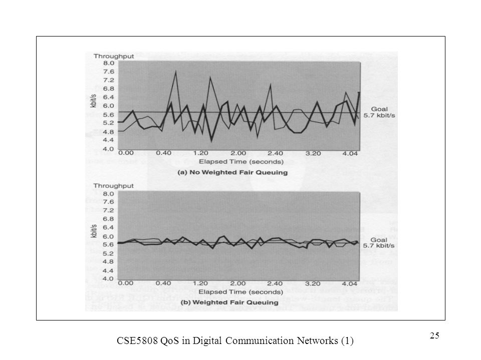


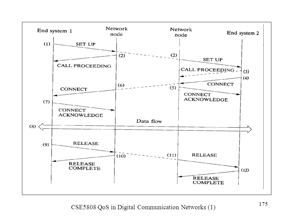


 Grants Chapter 6.>")


 Motion Controller Design for A Class of Second-order Systems Center for Self-Organizing Intelligent.>")

>")


>")

