1. R Graphics using the Grid Package Sigal Blay Statistical Genetics Working Group Dept. Of Statistics and Actuarial Science Simon Fraser University January 2006

2. Grid Low level graphics system Produces editable graphical components (not just graphics output) Object Oriented - graphical components can be reused and recombined

3. A standard set of graphical primitives: grid.rect(...) grid.lines(...) grid.polygon(...) grid.circle(...) grid.text(...) library(help = grid) for details

4. For every function of the form grid.* there is an equivalent function *Grob that returns a graphical object but doesn't draw it on the graphics device: grid.rect(...) rectGrob(...) grid.lines(...) linesGrob(...) grid.polygon(...) polygonGrob(...) grid.circle(...) circleGrob(...) grid.text(...) textGrob(..) Usage: Rect <- rectGrob(...) grid.draw(Rect)

5. Graphical output can be positioned and sized relative to a large number of coordinate systems grid.rect(x = unit(0, “native"), y = unit(1.5, “npc"), height = unit(0.5, "inches"), width = unit(0.8, “lines”)) help(unit) for details

6. Can specify various graphical parameters grid.rect(gp=gpar(col="red", lwd=2, fill="yellow", lty="dotted")) grid.text(gp=gpar(col="red", fontsize=10, fontface="italic")) help(gpar) for details

7. Working with viewports All drawing occurs in the current grid viewport, a defined rectangular region with it's own defined coordinate system: vp <- viewport(width=0.5, height=0.2, angle=45) grid.show.viewport(vp) help(viewport) for details

8. vp <- viewport(width=0.5, height=0.2, angle=45, name="VP") pushViewport(vp) grid.rect() popViewport()

9. vp <- viewport(width=0.5, height=0.2, angle=45, name="VP") pushViewport(vp) grid.rect() grid.xaxis() grid.yaxis()

10. vp <- viewport(width=0.5, height=0.2, angle=45, name="VP") pushViewport(vp) grid.rect() grid.xaxis() grid.yaxis() grid.text("viewport region", y = 0.9)

11. vp <- viewport(width=0.5, height=0.2, angle=45, name="VP") pushViewport(vp) grid.rect() grid.xaxis() grid.yaxis() grid.text("viewport region", y = 0.9) upViewport() grid.text("root region",y = 0.1)

12. vp <- viewport(width=0.5, height=0.2, angle=45, name="VP") pushViewport(vp) grid.rect() grid.xaxis() grid.yaxis() grid.text("viewport region", y = 0.9) upViewport() grid.text("root region",y = 0.1) grid.text("more text", vp="VP“ y=0.7)

13. Query the viewport tree > current.viewport() viewport[ROOT] > current.vpTree() viewport[ROOT]->(viewport[VP]) > downViewport("VP") > popViewport() > current.vpTree() viewport[ROOT]

14. Can push multiple viewport pushViewport(vpList(vp1, vp2, vp3)) Can push nested viewports pushViewport(vpStack(vp1, vp2, vp3)) pushViewport(vpTree(vp1, vpList(vp2, vp3))) Can integrate with a layout

15. plotViewport(...) a convenience function for producing a viewport with a central plot region surrounded by margins given in terms of a number of lines of text. dataViewport(...) a convenience function for producing a viewport with x- and/or y-scales based on numeric values passed to the function.

16. grid creates graphical objects ( grobs ): grid.rect(..., name="box") grid.circle(...) grid.edit("box", gp=gpar(fill="yellow")) grid.remove("box") 

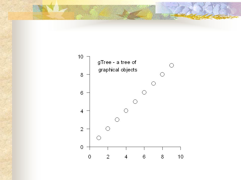
17. gTree – a tree of grobs vp<-viewport(..., name="view") x <- xaxisGrob(name = "axis1") y <- yaxisGrob(name = "axis2") points <- pointsGrob(1:9, 1:9, name="dataPoints") title <- textGrob(..., name="myTitle") tree <- gTree(name="Tree”, vp=vp, children=gList(x,y,title,points)) grid.draw(tree)

19. Query and edit a gTree > getNames() # list all top-level grobs [1] "Tree“ > childNames(tree) [1] "axis1" "axis2" "myTitle“ "dataPoints" > childNames(grid.get("Tree")) [1] "axis1" "axis2" "myTitle“ "dataPoints" > grid.add("Tree", grid.rect()) > grid.edit(gPath("Tree","dataPoints"), pch=2)

21. Example: LDheatmap package Plots measures of pairwise linkage disequilibria for SNPs

22. > getNames() [1] "ldheatmap" > childNames(grid.get("ldheatmap")) [1] "heatMap" "geneMap" "Key“ > childNames(grid.get("heatMap")) [1] "heatmap" "title" > childNames(grid.get("geneMap")) [1] "diagonal" "segments" "title" "symbols“ "SNPnames" > childNames(grid.get("Key")) [1] "colorKey" "title" "labels" "ticks” "box"

23. grid.edit("symbols", pch=20, gp=gpar(cex=2)) grid.edit(gPath("ldheatmap","heatMap","title"), gp=gpar(col="red")) grid.edit(gPath("ldheatmap","heatMap","heatmap“), gp=gpar(col="white", lwd=2)) 

24. Conclusion the R grid package enables the production of reusable and flexible graphical components

25. Further reading R Graphics / Paul Murrell