Download presentation
Presentation is loading. Please wait.

1
Environmental Data Analysis with MatLab
Lecture 6: The Principle of Least Squares

2
SYLLABUS Lecture 01 Using MatLab Lecture 02 Looking At Data Lecture 03 Probability and Measurement Error Lecture 04 Multivariate Distributions Lecture 05 Linear Models Lecture 06 The Principle of Least Squares Lecture 07 Prior Information Lecture 08 Solving Generalized Least Squares Problems Lecture 09 Fourier Series Lecture 10 Complex Fourier Series Lecture 11 Lessons Learned from the Fourier Transform Lecture 12 Power Spectra Lecture 13 Filter Theory Lecture 14 Applications of Filters Lecture 15 Factor Analysis Lecture 16 Orthogonal functions Lecture 17 Covariance and Autocorrelation Lecture 18 Cross-correlation Lecture 19 Smoothing, Correlation and Spectra Lecture 20 Coherence; Tapering and Spectral Analysis Lecture 21 Interpolation Lecture 22 Hypothesis testing Lecture 23 Hypothesis Testing continued; F-Tests Lecture 24 Confidence Limits of Spectra, Bootstraps

3
estimate model parameters using the principle of least-squares
purpose of the lecture estimate model parameters using the principle of least-squares Least-squares is a standard way to solve a linear model.

4
the least squares estimation of model parameters and their covariance
part 1 the least squares estimation of model parameters and their covariance Emphasize that calculating covariance is an integral part of the process. A answer is of no value without information about its accuracy. All estimates of model parameters based on noisy data are inherently uncertain. The key question is how uncertain.

5
motivates us to define an error vector, e
the prediction error motivates us to define an error vector, e This slide and the next three are review.

6
prediction error in straight line case
dipre ei data, d diobs Review the distinction between the observed and predicted data. Review how the error is calculated. auxiliary variable, x

7
total error single number summarizing the error
sum of squares of individual errors

8
principle of least-squares
that minimizes Remind students that the total error was defined in order to quantify what “about equal” means.

9
least-squares and probability
suppose that each observation has a Normal p.d.f. 2

10
for uncorrelated data the joint p. d. f
for uncorrelated data the joint p.d.f. is just the product of the individual p.d.f.’s least-squares formula for E suggests a link between probability and least-squares

11
now assume that Gm predicts the mean of d
Gm substituted for d minimizing E(m) is equivalent to maximizing p(d)
 is equivalent to maximizing p(d)")
12
the principle of least-squares determines the m that makes the observations “most probable” in the sense of maximizing p(dobs) Emphasize the strong link between two ways of thinking about goodness-of-fit, one involving error, the other involving probability.

13
the principle of least-squares determines the model parameters that makes the observations “most probable” (provided that the data are Normal) this is the principle of maximum likelihood
 this is the principle of maximum likelihood")
14
a formula for mest at the point of minimum error, E ∂E / ∂mi = 0 so solve this equation for mest

15
Result

16
where the result comes from
so

17
unity when k=j zero when k≠j since m’s are independent
use the chain rule so just delete sum over j and replace j with k unity when k=j zero when k≠j since m’s are independent

18
which gives

19
covariance of mest mest is a linear function of d of the form mest = M d so Cm = M Cd MT, with M=[GTG]-1GT assume Cd uncorrelated with uniform variance, σd2 then Show how many of the factors in the expression cancel one another.

20
two methods of estimating the variance of the data
prior estimate: use knowledge of measurement technique the ruler has 1mm tic marks, so σd≈½mm posterior estimate: use prediction error

21
posterior estimates are overestimates when the model is poor
reduce N by M since an M-parameter model can exactly fit N data

22
m=mest±2σmi (95% confidence)
confidence intervals for the estimated model parameters (assuming uncorrelated data of equal variance) so σmi = √[Cm]ii and m=mest±2σmi (95% confidence)
 so. σmi = √[Cm]ii. and. m=mest±2σmi (95% confidence)")
23
MatLab script for least squares solution
mest = (G’*G)\(G’*d); Cm = sd2 * inv(G’*G); sm = sqrt(diag(Cm)); Emphasize that this solution works regardless of the details of G. Explain use of backslash operator. Explain that the diag() function extracts the main diagonal from a matrix and puts it in a vector.
\(G’*d); Cm = sd2 * inv(G’*G); sm = sqrt(diag(Cm)); Emphasize that this solution works regardless of the details of G. Explain use of backslash operator. Explain that the diag() function extracts the main diagonal from a matrix and puts it in a vector.")
24
exemplary least squares problems
part 2 exemplary least squares problems

25
Example 1: the mean of data
the constant will turn out to be the mean

26
usual formula for the mean
variance decreases with number of data usual formula for the mean

27
2σd ± m1est = d = √N formula for mean formula for covariance
combining the two into confidence limits m1est = d = 2σd √N (95% confidence)
")
28
Example 2: fitting a straight line
intercept slope

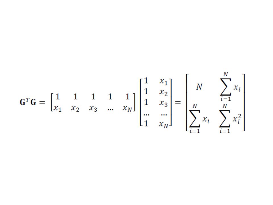
31
[GTG]-1= (uses the rule)
![[GTG]-1= (uses the rule)](http://slideplayer.com/slide/2343007/8/images/31/%5BGTG%5D-1%3D+%28uses+the+rule%29.jpg "[GTG]-1= (uses the rule)")
33
intercept and slope are uncorrelated when the mean of x is zero

34
keep in mind that none of this algrbraic manipulation is needed if we just compute using MatLab

35
Generic MatLab script for least-squares problems
mest = (G’*G)\(G’*dobs); dpre = G*mest; e = dobs-dpre; E = e’*e; sigmad2 = E / (N-M); covm = sigmad2 * inv(G’*G); sigmam = sqrt(diag(covm)); mlow95 = mest – 2*sigmam; mhigh95 = mest + 2*sigmam;
\(G’*dobs); dpre = G*mest; e = dobs-dpre; E = e’*e; sigmad2 = E / (N-M); covm = sigmad2 * inv(G’*G); sigmam = sqrt(diag(covm)); mlow95 = mest – 2*sigmam; mhigh95 = mest + 2*sigmam;")
36
Example 3: modeling long-term trend and annual cycle in Black Rock Forest temperature data d(t)obs d(t)pre error, e(t) time t, days Note that this plot has the observations, dobs, the “results”, dpre, and the error, e. The error large in the sense that it is an appreciable fraction of the amplitude of the data.
pre. error, e(t) time t, days. Note that this plot has the observations, dobs, the results , dpre, and the error, e. The error large in the sense that it is an appreciable fraction of the amplitude of the data.")
37
the model: long-term trend annual cycle
Identify m2 as the long-term slope. Note that the cosine and sine are paired.

38
MatLab script to create the data kernel
Ty=365.25; G=zeros(N,4); G(:,1)=1; G(:,2)=t; G(:,3)=cos(2*pi*t/Ty); G(:,4)=sin(2*pi*t/Ty); Ty is the number of days in a year, the period of the annual cycle.
; G(:,1)=1; G(:,2)=t; G(:,3)=cos(2*pi*t/Ty); G(:,4)=sin(2*pi*t/Ty); Ty is the number of days in a year, the period of the annual cycle.")
39
posterior variance of data based on error of fit σd = 5.60 deg C
prior variance of data based on accuracy of thermometer σd = 0.01 deg C posterior variance of data based on error of fit σd = 5.60 deg C You might discuss the rationale for using one of these estimates over the other. There are arguments both ways. The prior estimate is the better estimate of measurement noise. The posterior estimate more honestly reflects how well the model works (poorly). huge difference, since the model does not include diurnal cycle of weather patterns
. huge difference, since the model does not include diurnal cycle of weather patterns.")
40
long-term slope 95% confidence limits based on prior variance m2 = ± deg C / yr 95% confidence limits based on posterior variance m2 = ± deg C / yr in both cases, the cooling trend is significant, in the sense that the confidence intervals do not include zero or positive slopes. The key point if that the error bars do not overlap the m2=0, giving confidence to the assertion that the rate is negative.

41
However The fit to the data is poor, so the results should be used with caution. More effort needs to be put into developing a better model. Scientists should always be suspicious of models that only poorly fit the data.

42
covariance and the shape of the error surface
part 3 covariance and the shape of the error surface

43
solutions within the region of low error are almost as good as mest
4 m2 mest m1 m2est large range of m1 E(m) The error surface was shown in the previous lecture. Mention that it was computed via a grid search. mi miest small range of m2 near the minimum the error is shaped like a parabola. The curvature of the parabola controls the with of the region of low error
 The error surface was shown in the previous lecture. Mention that it was computed via a grid search. mi. miest. small range of m2. near the minimum the error is shaped like a parabola. The curvature of the parabola controls the with of the region of low error.")
44
near the minimum, the Taylor series for the error is:
You should skip this slide and the nest two if the class has too low a mathematical level to understand Taylor series. curvature of the error surface

45
starting with the formula for error
we compute its 2nd derivative

46
but so covariance of the model parameters
curvature of the error surface

47
the covariance of the least squares solution is expressed in the shape of the error surface
large variance small variance if you skipped the math, just asset the correspondence between variance and curvature of the error surface, E(m) E(m) mi mi miest miest
 E(m) mi. mi. miest. miest.")
Similar presentations