1. Copyright © 2011 by Pearson Education, Inc. All rights reserved Statistics for the Behavioral and Social Sciences: A Brief Course Fifth Edition Arthur Aron, Elaine N. Aron, Elliot Coups Prepared by: Genna Hymowitz Stony Brook University This multimedia product and its contents are protected under copyright law. The following are prohibited by law: -any public performance or display, including transmission of any image over a network; -preparation of any derivative work, including the extraction, in whole or in part, of any images; -any rental, lease, or lending of the program.

2. Copyright © 2011 by Pearson Education, Inc. All rights reserved Some Key Ingredients for Inferential Statistics Chapter 4

3. Copyright © 2011 by Pearson Education, Inc. All rights reserved Chapter Outline The Normal Curve Sample and Population Probability Normal Curves, Samples and Populations, and Probabilities in Research Articles

4. Copyright © 2011 by Pearson Education, Inc. All rights reserved Inferential Statistics Allow us to draw conclusions about theoretical principles that go beyond the group of participants in a particular study

5. Copyright © 2011 by Pearson Education, Inc. All rights reserved The Normal Curve Normal Distribution – histogram or frequency distribution that is a unimodal, symmetrical, and bell-shaped –a mathematical distribution –Researchers compare the distributions of their variables to see if they approximately follow the normal curve.

6. Copyright © 2011 by Pearson Education, Inc. All rights reserved Why the Normal Curve Is Commonly Found in Nature A persons ratings on a variable or performance on a task is influenced by a number of random factors at each point in time. These factors can make a person rate things like stress levels or mood as higher or lower than they actually are, or can make a person perform better or worse than they usually would. Most of these positive and negative influences on performance or ratings cancel each other out. Most scores will fall toward the middle, with few very low scores and few very high scores. –This results in an approximately normal distribution (unimodal, symmetrical, and bell-shaped).

7. Copyright © 2011 by Pearson Education, Inc. All rights reserved The Normal Curve and the Percentage of Scores Between the Mean and 1 and 2 Standard Deviations from the Mean There is a known percentage of scores that fall below any given point on a normal curve. –50% of scores fall above the mean and 50% of scores fall below the mean. –34% of scores fall between the mean and 1 standard deviation above the mean. –34% of scores fall between the mean and 1 standard deviation below the mean. –14% of scores fall between 1 standard deviation above the mean and 2 standard deviations above the mean. –14% of scores fall between 1 standard deviation below the mean and 2 standard deviations below the mean. –2% of scores fall between 2 and 3 standard deviations above the mean. –2% of scores fall between 2 and 3 standard deviations below the mean.

8. Copyright © 2011 by Pearson Education, Inc. All rights reserved The Normal Curve Table and Z Scores A normal curve table shows the percentages of scores associated with the normal curve. –The first column of this table lists the Z score –The second column is labeled % Mean to Z and gives the percentage of scores between the mean and that Z score. –The third column is labeled % in Tail.. Z% Mean to Z% in Tail.093.5946.41.103.9846.02.114.3845.62

9. Copyright © 2011 by Pearson Education, Inc. All rights reserved Using the Normal Curve Table to Figure a Percentage of Scores Above or Below a Raw Score If you are beginning with a raw score, first change it to a Z Score. –Z = (X – M) / SD Draw a picture of the normal curve, decide where the Z score falls on it, and shade in the area for which you are finding the percentage. Make a rough estimate of the shaded areas percentage based on the 50%–34%–14% percentages. Find the exact percentages using the normal curve table. –Look up the Z score in the Z column of the table. –Find the percentage in the % Mean to Z column or the % in Tail column. If the Z score is negative and you need to find the percentage of scores above this score, or if the Z score is positive and you need to find the percentage of scores below this score, you will need to add 50% to the percentage from the table. Check that your exact percentage is within the range of your rough estimate.

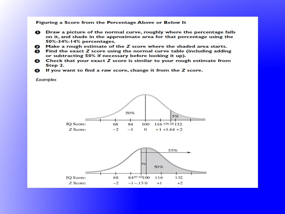
10. Copyright © 2011 by Pearson Education, Inc. All rights reserved Using the Normal Curve Table to Figure Z Scores and Raw Scores Draw a picture of the normal curve and shade in the approximate area of your percentage using the 50%–34%–14% percentages. Make a rough estimate of the Z score where the shaded area stops. Find the exact Z score using the normal curve table. Check that your Z score is within the range of your rough estimate. –From your picture, estimate the percentage of scores in the tail or between the mean and where the shading stops. To figure the percentage between the mean and where the shading stops, you will sometimes need to subtract 50 from your percentage. –Look up the closest percentage in the appropriate column of the normal curve table. –Find the Z score for that percentage. If you want to find a raw score, change it from the Z score. –X = (Z)(SD) + M

12. Copyright © 2011 by Pearson Education, Inc. All rights reserved Example of Using the Normal Curve Table to Figure Z Scores and Raw Scores: Step 1 Draw a picture of the normal curve and shade in the approximate area of your percentage using the 50%– 34%–14% percentages. –We want the top 5%. –You would start shading slightly to the left of the 2 SD mark.

13. Copyright © 2011 by Pearson Education, Inc. All rights reserved Example of Using the Normal Curve Table to Figure Z Scores and Raw Scores: Step 2 Make a rough estimate of the Z score where the shaded area stops. –The Z Score has to be between +1 and +2.

14. Copyright © 2011 by Pearson Education, Inc. All rights reserved Example of Using the Normal Curve Table to Figure Z Scores and Raw Scores: Step 3 Find the exact Z score using the normal curve table. –We want the top 5% so we can use the % in Tail column of the normal curve table. –The closest percentage to 5% is 5.05%, which goes with a Z score of 1.64.

15. Copyright © 2011 by Pearson Education, Inc. All rights reserved Example of Using the Normal Curve Table to Figure Z Scores and Raw Scores: Step 4 Check that your Z score is within the range of your rough estimate. – +1.64 is between +1 and +2.

16. Copyright © 2011 by Pearson Education, Inc. All rights reserved Example of Using the Normal Curve Table to Figure Z Scores and Raw Scores Check that your Z score is within the range of your rough estimate. –From your picture, estimate the percentage of scores in the tail or between the mean and where the shading stops. To figure the percentage between the mean and where the shading stops, you will sometimes need to subtract 50 from your percentage. –Look up the closest percentage in the appropriate column of the normal curve table. –Find the Z score for that percentage. If you want to find a raw score, change it from the Z score. –X = (Z)(SD) + M

17. Copyright © 2011 by Pearson Education, Inc. All rights reserved Example of Using the Normal Curve Table to Figure Z Scores and Raw Scores: Step 5 If you want to find a raw score, change it from the Z score. –X = (Z)(SD) + M –X = (1.64)(16) + 100 = 126.24

18. Copyright © 2011 by Pearson Education, Inc. All rights reserved How Are You Doing? Use the partial normal curve table found below to answer the following question: If the data from your study were normally distributed, what percentage of scores would fall between the mean and a Z score of.10? Z% Mean to Z% in Tail.093.5946.41.103.9846.02.114.3845.62

19. Copyright © 2011 by Pearson Education, Inc. All rights reserved Sample and Population Population –entire set of things of interest e.g., the entire piggy bank of pennies e.g., the entire population of individuals in the US Sample –the part of the population about which you actually have information e.g., a handful of pennies e.g., 100 men and women who answered an online questionnaire about health care usage

20. Copyright © 2011 by Pearson Education, Inc. All rights reserved Why Samples Instead of Populations Are Studied It is usually more practical to obtain information from a sample than from the entire population. The goal of research is to make generalizations or predictions about populations or events in general. Much of social and behavioral research is conducted by evaluating a sample of individuals who are representative of a population of interest.

21. Copyright © 2011 by Pearson Education, Inc. All rights reserved Methods of Sampling Random Selection –method of choosing a sample in which each individual in the population has an equal chance of being selected e.g., using a random number table Haphazard Selection –method of selecting a sample of individuals to study by taking whoever is available or happens to be first on a list This method of selection can result in a sample that is not representative of the population.

22. Copyright © 2011 by Pearson Education, Inc. All rights reserved Statistical Terminology for Sample and Populations Population Parameters –mean, variance, and standard deviation of a population –are usually unknown and can be estimated from information obtained from a sample of the population Sample Statistics –mean, variance, and standard deviation you figure for the sample –calculated from known information

23. Copyright © 2011 by Pearson Education, Inc. All rights reserved Probability Expected relative frequency of a particular outcome –outcome term used for discussing probability for the result of an experiment –expected relative frequency number of successful outcomes divided by the number of total outcomes you would expect to get if you repeated an experiment a large number of times long-run relative-frequency interpretation of probability –understanding of probability as the proportion of a particular outcome that you would get if the experiment were repeated many times

24. Copyright © 2011 by Pearson Education, Inc. All rights reserved Steps for Figuring Probability Determine the number of possible successful outcomes. Determine the number of all possible outcomes. Divide the number of possible successful outcomes by the number of all possible outcomes.

25. Copyright © 2011 by Pearson Education, Inc. All rights reserved Figuring Probability You have a jar that contains 100 jelly beans. 9 of the jelly beans are green. The probability of picking a green jelly bean would be 9 (# of successful outcomes) or 9% 100 (# of possible outcomes)

26. Copyright © 2011 by Pearson Education, Inc. All rights reserved Range of Probabilities Probability cannot be less than 0 or greater than 1. –Something with a probability of 0 has no chance of happening. –Something with a probability of 1 has a 100% chance of happening.

27. Copyright © 2011 by Pearson Education, Inc. All rights reserved p p is a symbol for probability. –Probability is usually written as a decimal, but can also be written as a fraction or percentage. –p <.05 the probability is less than.05

28. Copyright © 2011 by Pearson Education, Inc. All rights reserved Probability, Z Scores, and the Normal Distribution The normal distribution can also be thought of as a probability distribution. –The percentage of scores between two Z scores is the same as the probability of selecting a score between those two Z scores.

29. Copyright © 2011 by Pearson Education, Inc. All rights reserved Normal Curves, Samples and Populations, and Probability in Research Articles Normal curve is sometimes mentioned in the context of describing a pattern of scores on a particular variable. Probability is discussed in the context of reporting statistical significance of study results. Sample selection is usually mentioned in the methods section of a research article.

30. Copyright © 2011 by Pearson Education, Inc. All rights reserved Key Points In behavioral and social science research, scores on many variables approximately follow a normal curve which is a bell-shaped, symmetrical, and unimodal distribution. 50% of the scores on a normal curve are above the mean, 34% of the scores are between the mean and 1 standard deviation above the mean, and 14% of the scores are between 1 standard deviation above the mean and 2 standard deviations above the mean. A normal curve table is used to determine the percentage of scores between the mean and any particular Z score and the percentage of scores in the tail for any particular Z score. This table can also be used to find the percentage of scores above or below any Z score and to find the Z score for the point where a particular percentage of scores begins or ends. A population is a group of interest that cannot usually be studied in its entirety and a sample is a subgroup that is studied as representative of this larger group. Population parameters are the mean, variance, and standard deviation of a population, and sample statistics are the mean, variance, and standard deviation of a sample. Probability (p) is figured as the proportion of successful outcomes to total possible outcomes. It ranges from 0 (no chance of occurrence) to 1 (100% chance of occurrence). The normal curve can be used to determine the probability of scores falling within a particular range of values. Sample selection is sometimes discussed in research articles.