1. Complex Variables

2. Complex numbers are really two numbers packaged into one entity (much like matrices). The two “numbers” are the real and imaginary portions of the complex number:

3. We may plot complex numbers in a complex plane: the horizontal axis corresponds to the real part and the vertical axis corresponds to the imaginary part.
Im{z}
z = x + jy y
Re{z} x

4. Often, we wish to use polar coordinates to specify the complex number
Often, we wish to use polar coordinates to specify the complex number. Instead of horizontal x and vertical y, we have radius r and angle q.
Im{z}
z = x + jy y r
Re{z} q x

5. The best way to express a complex number in polar coordinates is to use Euler’s identity:
So,
and

6. We also have
A summary of the complex relationships is on the following slide.

7. Im{z} r
y = r sin q q
Re{z}
x = r cos q

8. The magnitude of a complex number is the square-root of the sum of the squares of the real and imaginary parts:
If we set the magnitude of a complex number equal to a constant, we have

9. or,
This is the equation of a circle, centered at the origin, of radius c.

10. Im{z}
c2 = |z|2 = x2 + y2
z = x + jy y c
Re{z} x

11. Suppose we wish to find the region corresponding to
This would be a disk, centered at the origin, of radius c.

12. Im{z}
x2 + y2 = |z|2 < c2 y c
Re{z} x

13. Suppose we wish to find the region corresponding to
This would be a disk, centered at z0, of radius c.

14. Im{z}
(x-x0)2 + (y-y0)2 = |z-z0|2 < c2 = |z-z0|2 c y0 z0
Re{z} x0

15. Functions of Complex Variables
Suppose we had a function of a complex variable, say
Since z is a complex number, w will be a complex number. Since z has real and imaginary parts, w will have real and imaginary parts.

16. The standard notation for the real and imaginary parts of z are x and y respectively.
The standard notation for the real and imaginary parts of w are u and v respectively.

17. where
Both u and v are functions of x and y.

18. So a complex function of one complex variable is really two real functions of two real variables.

19. Exercise: Find u(x,y) and v(x,y) for each of the following complex functions:

20. Continuity of Complex Functions
In order to perform operations such as differentiation and integration of complex functions, we must be able to verify of the complex function is continuous.
A complex function
is said to be continuous at a point z0 if as z approaches z0 (from any direction) then f(z) can be made arbitrarily close to f(z0).

21. A more mathematical definition of continuity would be for any e, we can make
for some d such that
Since we are dealing with complex numbers, the geometric interpretation of this statement is different from that of real numbers.

22. The region |z-z0| < d defines a disk in the complex plane of radius d centered about z0.
Im{z} z0
Re{z}

23. So, if we wish |f(z)-f(z0)| < e we must find a d to make this so.
Im{w}
f(z0)
Re{w}

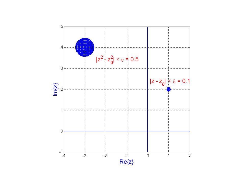
24. Example: Suppose
Find d such that
for

25. Solution:

26. All we need to do is to find a value of d such that if
then

27. We can do some calculations on a spreadsheet (continuity.xls).
A value of d < 0.1 seems to do it.

28. A MATLAB plot (by continuity
A MATLAB plot (by continuity.m) of the previous example is shown on the following slide.

30. Differentiation of Complex Functions
How do we take derivatives of complex functions with respect to complex variables? If
what is

31. The differential dz can vary in one of two ways: along the real axis (dx) or along the imaginary axis (dy).
Im{z}
y+dy dy y dx
Re{z} x
x+dx

32. As z varies in either direction, the derivative must be the same.
x direction
y direction
So, we must have

33. These last two conditions
are called the Cauchy-Riemann equations. These equations are the criteria for a complex function to be differentiable (with respect to z = x + jy).

34. Example: Show that the function
is differentiable
Solution: We have shown that

36. Now that we have determined that this function is differentiable, the derivative can be found usingor

37. If we apply these formulas to
where

38. we have or

39. We see that the derivative in both cases is
The answer is what we would expect to get if z were treated as a real variable.
As it turns out, for most well-behaved complex functions, the derivative can be found by treating z as if it were a real variable.

40. Example: Show that the function
is not differentiable
Solution: We have shown that

42. Exercise: Is
differentiable?

43. Definition: A function
is said to be analytic if it is differentiable throughout a region in the complex plane.

44. Integration of Complex Functions
What happens when we try to take the integral of a complex function along some path in the complex plane?

45. A complex integral is like a line integral in two dimensions.
The real and the imaginary parts of the integral are nearly identical to classic line integrals.

46. Example: Integrate
over the real interval z = 0 + j0 to z = 2 + j0.
Solution: We have shown that

48. Since we are integrating along the real (x) axis, all integrals with respect to dy are zero. In addition y=0. So,

49. The result is exactly what we would expect to get if we simply integrated a real variable from 0 to 2.

50. Example: Integrate
over the imaginary interval z = 0 + j0 to z = 0 + j2.
Solution: The integral becomes

51. The result is exactly what we would expect to get if we simply integrated
where C = jy and where y=[0,2] :

52. over the complex path z = 0 + j2 to z = 2 + j2.
Example: Integrate
over the complex path z = 0 + j2 to z = 2 + j2.
Im{z} 2 2
Re{z}

53. Solution:
The value of y is that of the path: y=2.

55. over the complex path z = 2 + j0 to z = 2 + j2.
Example: Integrate
over the complex path z = 2 + j0 to z = 2 + j2.
Im{z} 2 2
Re{z}

56. Solution:

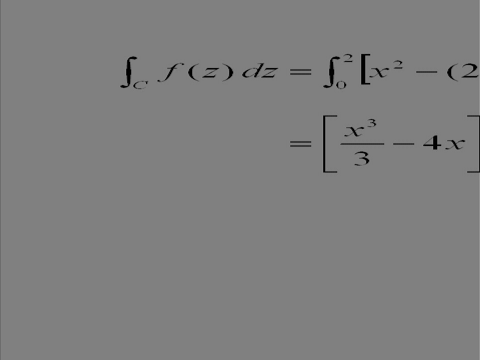
57. over the complex path z = 0 + j0 to z = 2 + j2.
Example: Integrate
over the complex path z = 0 + j0 to z = 2 + j2.
Im{z} 2 2
Re{z}
Solution: The path of integration is a line z = x + jy where x = y = t = [0,2].

58. Solution: The integral is more complicated.

60. This result is the same as the sum of the integral from 0+j0 to 0+j2 with the integral from 0+j2 to 2+j2.
Im{z} 2 2
Re{z}

61. This result also is the same as the sum of the integral from 0+j0 to 2+j0 with the integral from 2+j0 to 2+j2.
Im{z} 2 2
Re{z}
So it seems that it does not matter what path is taken as long as the endpoints are the same.

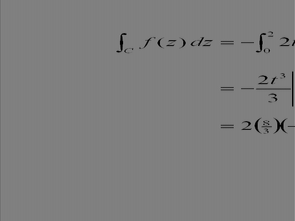
62. Example: Integrate
over two paths:
(1) a semicircle z = ejq, where q = [0,p].
(2) a semicircle z = e-jq, where q = [0,p].
Show that the two integrals are the same.

63. Im{z} C1
Re{z}
q = 0
q = p C2

64. Solution: This integration is best handled using polar coordinates:

65. The integral around curve C1 is

66. The integral around curve C2 is

67. If we were to integrate around the whole circle C = ejq for q = [0, 2p], we would get
The curve C can be thought of as C1 + (-C2 ).

68. Cauchy’s Integral Theorem: If a function f(z) is analytic over a region R enclosed by a (closed) path C, then
Im{z} C R
Re{z}

69. Simple Proof:
Both integrals are line integrals around a closed curve C. We can apply Green’s theorem (a special case of Stoke’s theorem) to these line integrals

70. If f(z) is analytic, then the Cauchy-Riemann equations apply:
If these are true, then both integrands of
are zero and the theorem is proved.

71. If
and C = C1 + C2, then

72. Im{z} C1 C2
Re{z}

73. We also have

74. Im{z} C1
-C2
Re{z}

75. So it does not matter what path that you take so long as the endpoints are the same provided f(z) is analytic between any of the two paths.
If f(z) is not analytic at some point between two paths, then the path does matter.

76. over a unit circle z = ejq, where q = [0,2p].
Example: Integrate
over a unit circle z = ejq, where q = [0,2p].
Im{z}
Re{z}

77. Solution: As with the previous example, this integration is best handled using polar coordinates:

78. This integral is not zero because there is a discontinuity (actually a pole) at z = 0.

79. over a unit circle z = 1 + ejq, where q = [0,2p].
Example: Integrate
over a unit circle z = 1 + ejq, where q = [0,2p].
Im{z}
Re{z}

80. Solution: Let us first write the integral.
To carry-out this integration, we first perform a substitution of variables. Let z = z-1.

81. The path C’ is equal to C minus one:
Im{z} C’ C
Re{z}
We see that

82. This integral is not zero because there is a discontinuity (a pole) at z = 1 or z = 0.

83. Exercise: Show that no matter what z0 is, if C is a circular path (of any radius) around z0 we will have

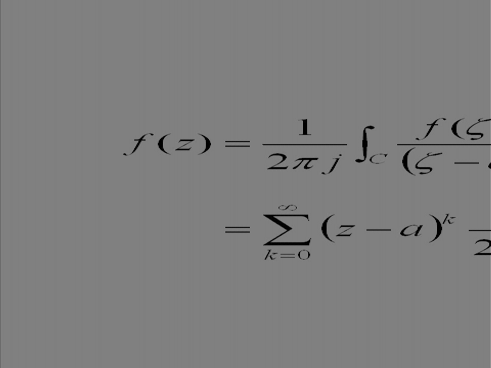
84. Cauchy’s Integral Formula: Let f(z) be analytic over a region R enclosed by a closed path C. If z0 is a point within R, then
Note that while f(z) is analytic throughout R,
f(z)/(z-z0 ) is not analytic (z0 is a pole).

85. Im{z} C R z0
Re{z}

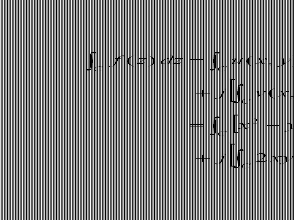
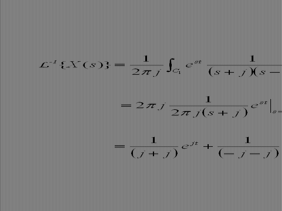
86. Proof: We add and subtract f(z0) to the numerator of the integrand so as to split-up the integral into two terms:

87. If f(z) is analytic within the region R, then it is also continuous
If f(z) is analytic within the region R, then it is also continuous. So, for any e, we can find a d such that for
we have
Let us choose a r < d such that z  R, i.e., the disk |z-z0| < r is totally within R. Let denote the path |z-z0| = r by the symbol C’ .

88. r
Im{z} C R z0 C’
Re{z}

89. So if
and

90. So for appropriate values of d and r, the integrand in
can be made arbitrarily small. Now since the integrand is analytic except at z = z0, we have

91. The integral
is equal to 2pj. So,
and the theorem is proved.

92. Example: Evaluate the integral
where C is a closed curve around z = 1.
Solution:
So,

93. The formula
makes calculating derivatives with respect to z0 relatively easy. We do not have to worry about z: it is independent of z0.

94. In general it can be shown that
This formula is very useful in deriving the Taylor series.

95. Example: Evaluate the integral
where C is a closed curve around z = 1.
Solution:
So,

96. Example: Evaluate the integral
where C is a closed curve around z = 1.
Solution:
So,

97. Example: Evaluate the integral
where C is a closed curve around z = 2.
Solution:

98. Exercise: Evaluate the integral
where C is a closed curve around z = 1.

99. Inverse Laplace Transforms
We used a formula to calculate the forward Laplace transform, but we did not use a formula to calculate the inverse Laplace transform. Such a formula exists!
The forward Laplace transform was found using

100. The inverse Laplace transform can be found using a complex inversion integral formula:
We can evaluate the inverse Laplace transform using Cauchy’s integral formula.

101. Cauchy’s integral formula is for an integration around a closed loop
Cauchy’s integral formula is for an integration around a closed loop. The inverse Laplace transform formula is an integral along an infinite line. This infinite line integral can actually be thought of as a loop.
Let us construct a closed curve C consisting of a line along the imaginary axis and a semicircle in the left-half plane.

102. Im{s}
s  +j r
s  -
Re{s} C
s  -j

103. As the radius r of the semicircle approaches infinity, the closed loop approaches an infinite line (from s = -j to +j). As r approaches infinity, both the semicicular curve and the infinite line pass through something called the point at infinity.
The point at infinity can be reached from either the positive or negative half of the real or the imaginary axis. The limits s  +j, s  -j and s  - are all the same.

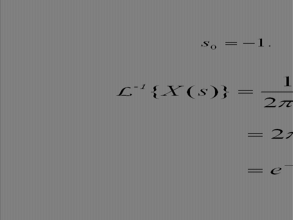
104. Example: Find the inverse Laplace transform of
Solution:

106. Example: Find the inverse Laplace transform of
Solution:

107. The integral can be evaluated in the complex plane about a curve C:
The curve C is an extension of the s= -j to s = +j line.

108. Im{s}
Re{s} C

109. There are actually two points of discontinuity:
We can evaluate the complex inversion integral by evaluating the integral around these two points of discontinuity. Let us call the paths around these two points C1 and C2.

110. Im{s} C1
s0 = +j
Re{s} C2 C
s0 = -j

112. Exercise: Using the complex inversion integral, find the inverse Laplace transforms of the following functions:
(First find the points of discontinuity and then evaluate the integral in paths around these points.)

113. Example: Find the inverse Laplace transform of
Solution:

114. There is one point of discontinuity:

115. Sequences and Series Consider the sequence of values
each term in this sequence can be represented by

116. What happens as n goes to infinity? For this example zn goes to zero.
How about the sequence of values
each term in this sequence can be represented by

117. This sequence is said to converge to two (2): as n goes to infinity, zn goes to two.
How about the sequence of values
This series does not converge to any value, but rather it is said to diverge.

118. This sequence {zn } is said to converge to a value c if zn can be made arbitrarily close to c for a large enough value of n.
A more formal definition of convergence of series would be for any positive value e, we can find an integer N such that for
we must have

119. The expression
is for a complex number zn and defines a disk in the complex plane. e
Im{z} c
Re{z}

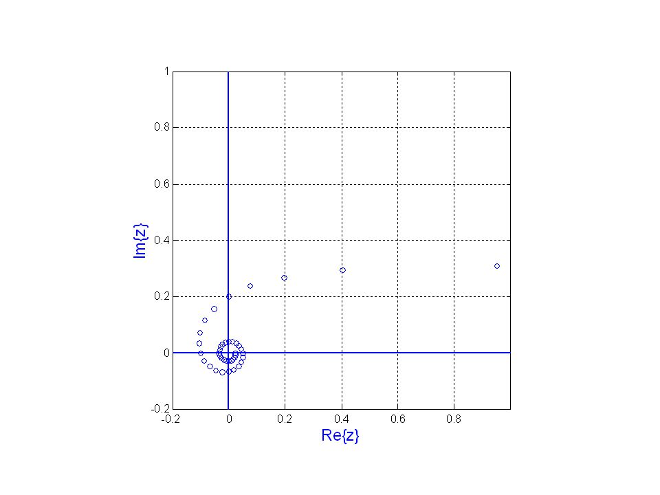
120. Example: Plot the sequence of values in
in the complex plane
Solution: The radius of zn is 1/n and the angle of zn is 2pn/20. The plot is performed using MATLAB (sequence.m) and is shown on the following slide page.

122. This sequence converges to zero
This sequence converges to zero. The relationship between the sequence index n and distance to the limit is rather easy in this case.
For
we must have
where 1/e corresponds to the smallest integer greater than 1/e.

123. Similarly, for
we must have

124. A necessary (but not sufficient) condition for a sequence to converge is that it be bounded. A bounded sequence is {zn } is one that for all n we have
for some finite value B. If a sequence is not bounded, it will diverge.

125. Just because a sequence is bounded does not mean it converges
Just because a sequence is bounded does not mean it converges. Many sequences which are bounded do not converge. For example,
For this sequence

126. zn n 1 2 3 4 5

127. While this sequence does not have a limit, it does have an upper bound (+1) and a lower bound (-1) as n   . These “bounds” are called the supremum and the infimum respectively. The supremum is the smallest upper bound (+1) and the infimum is the largest lower bound (-1). These bounds are abbreviated sup and inf respectively.

128. Note that while {zn } does not converge, there are subsequences
that do converge.

129. Series Suppose we were to add the numbers in a sequence:
The term sn is called the partial sum of the series {zn }. The summation is a series.

130. If we were to take the limit as n   , we would get an infinite series:
If the sequence of partial sums converges, we say that the series converges.

131. A necessary (but not sufficient) condition for the series {sn } to converge is that the sequence {zn } converges. The series is generally “wilder” that the sequence. If the series converges, the sequence must necessarily converge. If the series diverges, the sequence may or may not converge.

132. Example: Consider the (convergent) sequence
The corresponding series does not converge (as n goes to infinity):

133. Now how do we find sufficient conditions for a series to converge
Now how do we find sufficient conditions for a series to converge? There are five (5) standard tests for series convergence:
(1) Comparison Test: compare series term-by-term against a known convergent series.
(2) Geometric Series Test: a geometric series converges if each geometric term is less than one

134. (3) Ratio Test: Take the limit of the ratio of one term to the previous term. If the limit is less than one, the series converges
(4) Root Test: Take the k-th root of the k-th term. If the limit is less than one, the series converges.
(5) Integral Test: compare the sequence to an integrand of a known integral.

135. (1) Comparison Test: compare series term-by-term against a known convergent series.
If we have a known convergent series
then any series

136. such that
also converges.

137. (2) Geometric Series Test: a geometric series converges if each geometric term is less than one
A geometric series is of the form
We can use this form to find a closed-form expression for the geometric series

139. So,
If the geometric term q is such that qn goes to zero as n goes to infinity, then

140. In order for qn to go to zero, we must have
If q > 1, then the series diverges.

141. Example: Suppose q = ½.

142. Example: Suppose q = 9/10.

143. Example: Suppose q = -1/2.

144. (3) Ratio Test: Take the limit of the ratio of one term to the previous term. If the limit is less than one, the series converges If
then we take

145. If
then the series converges.

146. As a justification (hardly a proof) for this test, consider definining zk in terms of wk:

147. The term

148. If
then the series behaves like a convergent geometric series:

149. Example: Determine if
converges.
Solution: Taking the ratio test
We see that the series converges.

150. (4) Root Test: Take the k-th root of the k-th term
(4) Root Test: Take the k-th root of the k-th term. If the limit is less than one, the series converges. If
then we take

151. If
then the series converges.

152. As a justification (better than that of the ratio test but still not a proof) for this test, consider
If wk < 1, then the series is a convergent geometric series.

153. Example: Determine if
converges.
Solution: Taking the root test
We see that the series diverges. (ek dominates k2.)

154. (5) Integral Test: compare the sequence to an integrand of a known integral.
The term zk is really a function of k. We can represent that function as z(k) or z(x). The convergence of the integral
can be used to determine whether or not the series converges.

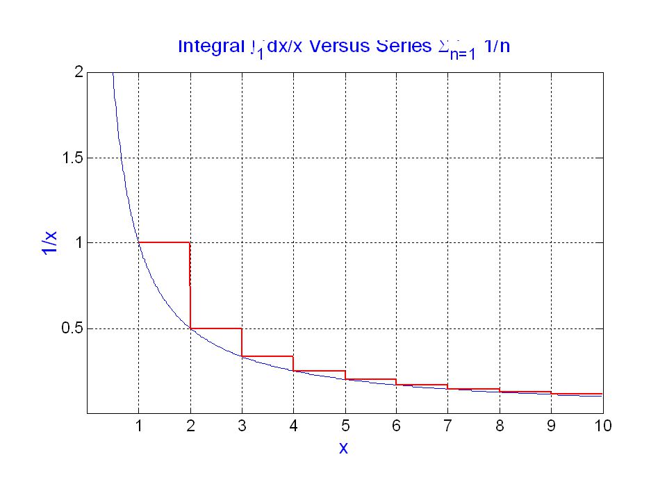
155. Example: Consider the series
This series is greater than the integral
Since the integral diverges [ln n], the series diverges.

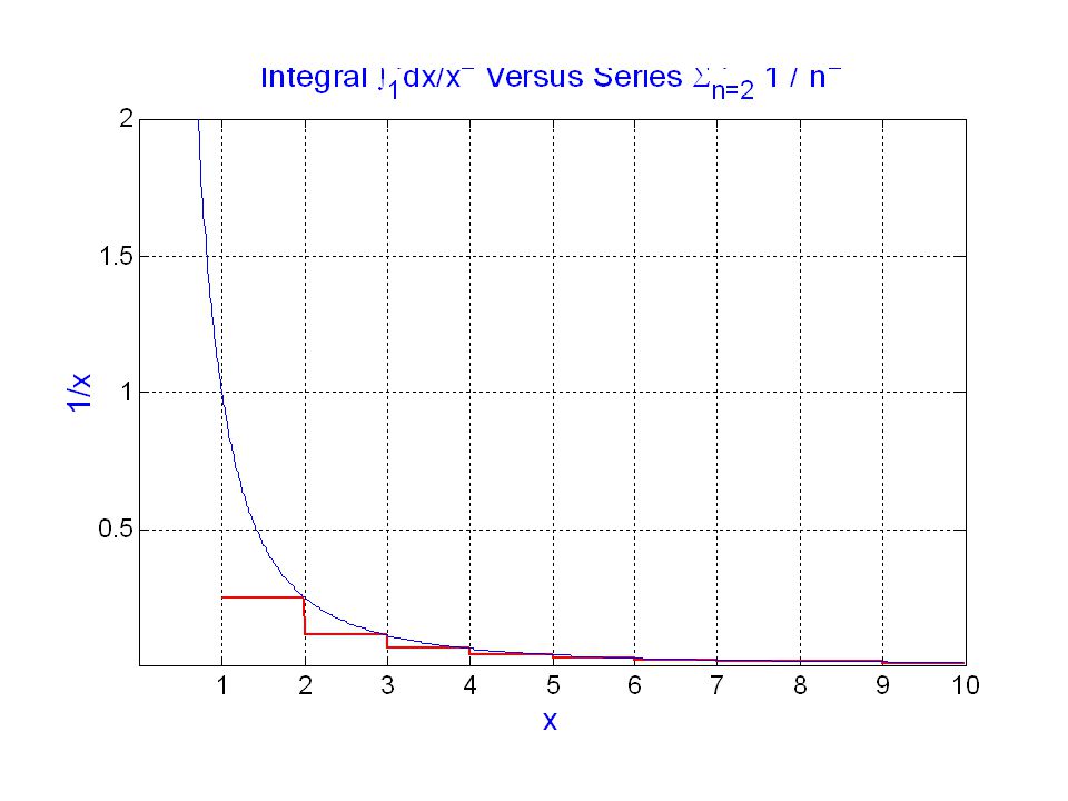
157. Example: Consider the series
This series from k=2 to k=n is less than the integral
Since the integral converges [1/n], the series converges.

159. Taylor Series
A Taylor series is a power series representation for a function.
A Taylor series is much like a Fourier series (which is a harmonic series).

160. To find a Taylor series, all we need to do is find the coefficients (much like Fourier series).
To find these coefficients let us start with Cauchy’s integral formula:
We will attempt to express this formula in a power series about z = a.

161. We start with the fraction in the integral:
The object is to express this in terms of powers of (z – a). So, we try to get this fraction in the form of an infinite geometric series:

162. The last is true if z is on a curve C at a distance r from a and z is within the close curve.

163. r
Im{z}
z is on C a z
Re{z}

165. The coefficient of (z – a)k inside the summation
is similar to the k-th derivative of f(a) from the corollary to Cauchy’s integral theorem:

166. So,
Hence, we have our Taylor series coefficients.

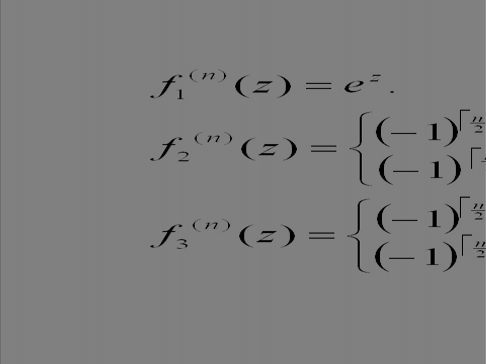
167. Example: Find the Taylor series for

169. We will evaluate the Taylor series about z = 0 :

170. So,

171. You can use these Taylor series to prove

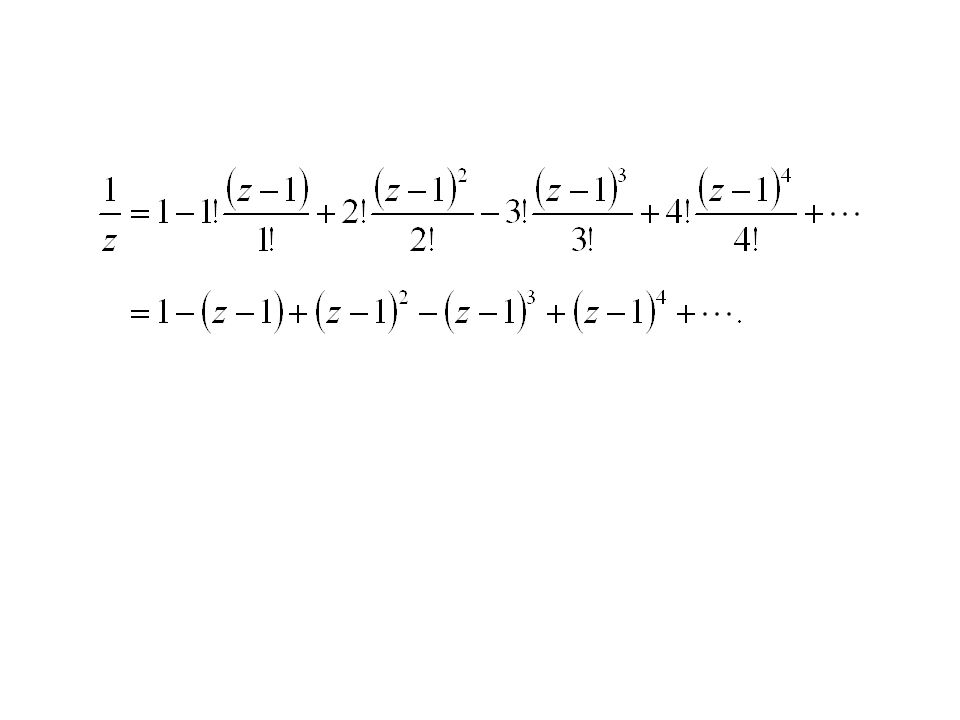
172. Example: Find the Taylor series for
Here, we will evaluate the series about a = 1.

174. Example: Find the Taylor series for
Here, we will evaluate the series about a = 1.

175. If z is not close to one, this series is very slow to converge.

176. Exercise: Find the Taylor series for
Evaluate the series about an arbitrary a.

177. Conformal Mapping
How do we “graph” complex functions? The difficulty lies in the dimensionality: we have two independent variables (x,y) and two dependent variables (u,v).

178. To “graph” this function, we start with a family of curves corresponding to constant values of x and constant values of y. These curves are represented by dashed green lines on the following slide.

179. y = Im{z}
y=4
y=3
y=2
y=1
x = Re{z}
x=1
x=2
x=3
x=4

180. To what do these curves correspond to in the u-v plane?
Let us start with a simple example

181. v = Im{w}
y=2
y=1
u = Re{w}
x=1
x=2

182. Example: Find the conformal map for
We expand ez from the real and imaginary parts of z.

183. This expansion is best handled using polar coordinates.
where

184. The resultant curves will be a set of circles of radii ex
The resultant curves will be a set of circles of radii ex. Constant values of y correspond to rays at angle y.

185. v = Im{w}
y=2
y=1
u = Re{w}
x=1
x=2

186. Negative values of x correspond to circles of radius e-|x|
Negative values of x correspond to circles of radius e-|x|. Negative values of y correspond to rays at angle -|y|.

187. v = Im{w}
x = -2
x = -1
u = Re{w}
x=2
y = -2
y = -1

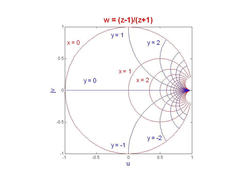
188. Example: Find the conformal map for
We represent z and w in terms of their real and imaginary components:

189. We then try to make the denominator real:

190. A plot of the constant x and the constant y curves (in the u-v plane) is shown on the following slide.

192. The resultant graph is that of a Smith Chart
The resultant graph is that of a Smith Chart. This chart is used in radio-frequency electronics. The graph is a conformal map of line impedance onto complex reflection coefficient.

193. The Argument Principle
Let
be a function of the complex variable z.
As z follows a path in the z-plane, what path does w follow in the w-plane?

194. Let z follow a closed path in the z-plane.
Im{z} C
Re{z}

195. As z follows this closed path, what path will w=f(z) follow?
As an example, let
As z goes around the circle once, w goes around the same circle twice.

196. Im{z}
Im{w} C C’
Re{z}
Re{w}

197. As another example, let
As z goes around the circle counter-clockwise, w goes around the same circle clockwise.

198. Im{z}
Im{w} C
Re{z}
Re{w} C’

199. Let us choose two points on the z-path: z1 and z2
Im{z} C z1
Re{z} z2
The two points z1 and z2 are very close together; their radii are the same, but their angles are different.

200. The two points z1 and z2 are very close together; their radii are the same, but their angles are different.

201. The corresponding points in the w-plane f(z1 ) and f(z2 ) are very close together. Like z, the radii of f(z1 ) and f(z2 ) are the same, but their angles are different.

202. As z follows the circular closed path, what path will f(z) follow?
To get an idea of the path f(z) will follow, let us look at log f(z).

203. The difference between log w1 and log w2 is

204. Now log w can be written as an indefinite integral:
The difference between log w1 and log w2 can be written as a definite integral:

205. The points 1 and 2 in the integral
correspond to z1 and z2. So,

206. Combining this expression with
we have

207. So, the integral from z1 to z2 is the same as the integral around the closed curve in the z-plane.
To summarize, as z follows a closed path in the z-plane, w=f(z) follows a closed path in the w-plane. The angular rotation that w takes is equal to f2 – f1.

208. Since w=f(z) follows a closed path in the w-plane, the angular rotation, f2 – f1, must be an integral multiple of 2p.

209. Suppose G(s) is a polynomial fraction:
Let s take on an infinite circular path in the right-half complex plane.

210. Im{s}
s  +j r
s  +
Re{s} C
s  -j

211. What kind of path will G(s) take?
To answer this question, let us try to evaluate the integral
where C is the curve described on the previous slide.

212. We will try to evaluate this integral by removing poles and zeroes in the right-half plane. Suppose p1 is a right-half plane pole. We can define a new function H(s) with this pole removed:
So,

213. If
we have

214. If
and
we have

215. The integral of
is equal to

216. By the Cauchy Integral Formula, the integralSo

217. Now suppose z1 is a right-half plane zero
Now suppose z1 is a right-half plane zero. We can define a new function F(s) with this zero removed:
So,

218. If
we have

219. If
and
we have

220. The integral of
is equal to

221. By the Cauchy Integral Formula, the integralSo

222. If we continue eliminating poles and zeroes, we get a term of -2pj for every pole and a term of +2pj for every zero. So
where Z is the number of zeroes, and P is the number of poles.

223. Now from our previous result,
we see that
where N is the number of rotations of G(s), Z is the number of right-half plane zeroes, and P is the number of right-half plane poles.

224. By looking at the number of clockwise rotations of G(s), we can find the number of right-half plane zeroes minus the number of right-half plane poles.
We have already done two examples:

225. We have already done two examples:
The first function did two counter-clockwise rotations for each counter-clockwise rotation of z.
The second function did one clockwise rotation for each counter-clockwise rotation of z.

226. Equivalently, for
The first function will do two clockwise rotations for each clockwise rotation of s. These clockwise rotations correspond to two zeroes (at zero).
The second function will do one counter-clockwise rotation for each clockwise rotation of s. This counter-clockwise rotation corresponds to one pole (at zero).

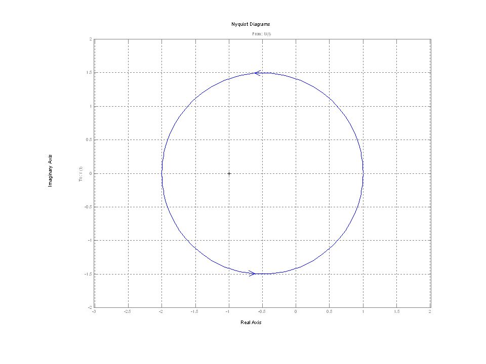
227. Example: How many times does the following transfer function circle the origin as s goes from -j to +j ?
Solution: There is one RHP pole and no RHP zeros (The term s+2 corresponds to a LHP zero: s = -2.) The plot of G(s) will circle the origin in the counter-clockwise direction once.

228. In MATLAB, we can plot G(s) using the control function nyquist().
>> EDU» s = tf('s');
>> H = (s+2)/(s-1);
>> nyquist(H)
The Nyquist plot is on the following slide.

230. In control systems, we are often concerned about the poles of a closed-loop transfer function
The poles of T(s) are the zeros of 1+G(s).
The right-half plane poles of T(s) are the right-half plane zeros of 1+G(s).

231. If we did a plot of
and 1+G(s) had no right-half plane poles, then the number of clockwise rotations around the origin is equal to the number of right-half plane zeros of 1+G(s) or the number of right-half plane poles of T(s) .

232. The number of clockwise rotations around the origin of
is equal to the number of clockwise rotations of
around s = -1.

233. Therefore, if 1+G(s) has no right-half plane poles, the number of clockwise rotations around s = -1 of
is equal to the number right-half plane poles of