1. Basic Probability

2. Frequency Theory A mathematical approach to making the notion of chance rigorous. Best applied to processes which can be repeated many times, independently, and under the same conditions. – Coin tossing – Dice rolling (craps) – Card games (blackjack, poker, etc.)

3. Probability

4. A few basic facts

5. Canonical Example

7. If you choose two tickets at random, what is the probability that both are labeled 3? – The answer depends on whether or not you replace the first ticket you draw. – However, the math you use to find the answer does not.

8. Multiplication Rule The probability that two events will both happen equals the probability of the first event multiplied by the probability of the second event given that the first event happened. P( A and B ) = P( A ) x P( B given A ) The probability P( B given A ) is called a conditional probability. Its sometimes written P( B | A ).

9. Drawing without replacement

10. Drawing with replacement

11. Independence Two events are said to be independent if the probability of the second event does not depend on the outcome of the first event. – That is, if P( B given A ) = P( B ) When drawing tickets at random with replacement, the draws are independent. Without replacement, the draws are dependent.

12. Examples A fair coin is tossed twice. If the second toss is heads, you win a dollar. – If the first toss is heads, what is your chance of winning a dollar? – If the first toss is tails, what is your chance of winning a dollar? The events first toss is heads and second toss is heads are independent.

13. Examples Two cards are dealt off the top of a well- shuffled deck of 52 standard playing cards. – What is the probability that the second card is the queen of hearts? – What is the probability that the second card is the queen of hearts given that the first card is a spade? The events drawing the queen of hearts and drawing a spade are dependent.

14. Warnings Use caution when multiplying probabilities. In general, P( A and B ) = P( A ) x P( B given A ). Only if A and B are independent is it true that P( A and B ) = P( A ) x P( B ). Dont apply the theory outlined above to unique events – events that cant be repeated many times, independently and under the same conditions. – What is the probability that tomorrows high temperature is 73 degrees Fahrenheit?

15. Activity: The Law of Averages Perform 50 coin flips. – For each flip, if the coin lands with heads showing, record a 1. If tails is showing, record a 0. Bring me the following data: – The total number of heads – The longest run of heads or tails – The number of runs of 4 heads (Note: a run of 5 heads = 2 runs of 4, a run of 6 heads = 3 runs of 4, etc.) – The number of times a head followed a run of 4 heads – Number of heads before the first tail. – Number of heads after the last tail.

16. John Kerrichs results Number of TossesNumber of headsDifference from expected 50250 10044-6 20098-2 300146-4 400199 5002555 60031212 70036818 80041313 9004588 10005022 2000101313

17. John Kerrichs results Number of TossesNumber of headsDifference from expected 3000151010 4000202929 5000253333 600030099 7000351616 8000403434 9000453838 10,000506767 In first 2000 tosses, there were 130 runs of 4 heads. In 69 cases the run was followed by a head, in 61 cases, it was followed by a tail.

18. Key takeaway points As the number of tosses increases, so does |(# heads) – (expected # of heads)| but the percentage difference decreases. The number of heads differs from the expected number due to chance variability. If the experiment is repeated, the number of heads is likely to be different. Runs dont change the probability of the next toss. (Tosses are independent events.)

19. Box Models

20. Modeling Chance Processes How many heads do you get if you toss a coin many times? How much money does a casino make on roulette? How accurate is a sample survey? These questions are about chance processes.

21. Box Models General strategy for analyzing chance processes: – Find an analogy between the process youre interested in and drawing numbers at random from a box. – Connect the variability you want to know about with the chance variability in the sum of the numbers drawn.

22. Box Models Three key questions – What numbers go into the box? – How many of each number? – How many draws?

23. Roulette

24. Box models for Roulette Example 1: Betting $1 on red. – Numbers in the box: +1, -1 (win pays even money) – How many of each: 18 tickets: +1, 20 tickets: -1 – Number of draws: the number of plays – We draw at random, with replacement The sum of the draws is your net gain. Ten plays: R R R B G R R B B R Ten draws: +1 +1 +1 -1 -1 +1 +1 -1 -1 +1 Net gain: +2

25. Box models for Roulette Example 2: Betting $1 on a single number – Numbers in the box: +35, -1 (win pays 35 to 1) – How many of each: 1 ticket: +35, 37 tickets: -1 – Number of draws: number of plays – We draw with replacement.

26. A box model in statistics A political candidate wants to enter a primary in a district with 100,000 eligible voters, but only if he has a good chance of winning. He hires a survey organization which samples 2500 voters. In the sample, 1328 favor the candidate. How far off is the survey likely to be? – Numbers in the box: 1 (vote for), 0 (vote against) – How many of each: unknown, 100,000 total – Number of draws: 2500 – We draw without replacement. – Sum of draws: number of votes for the candidate (1328)

27. Expected Value

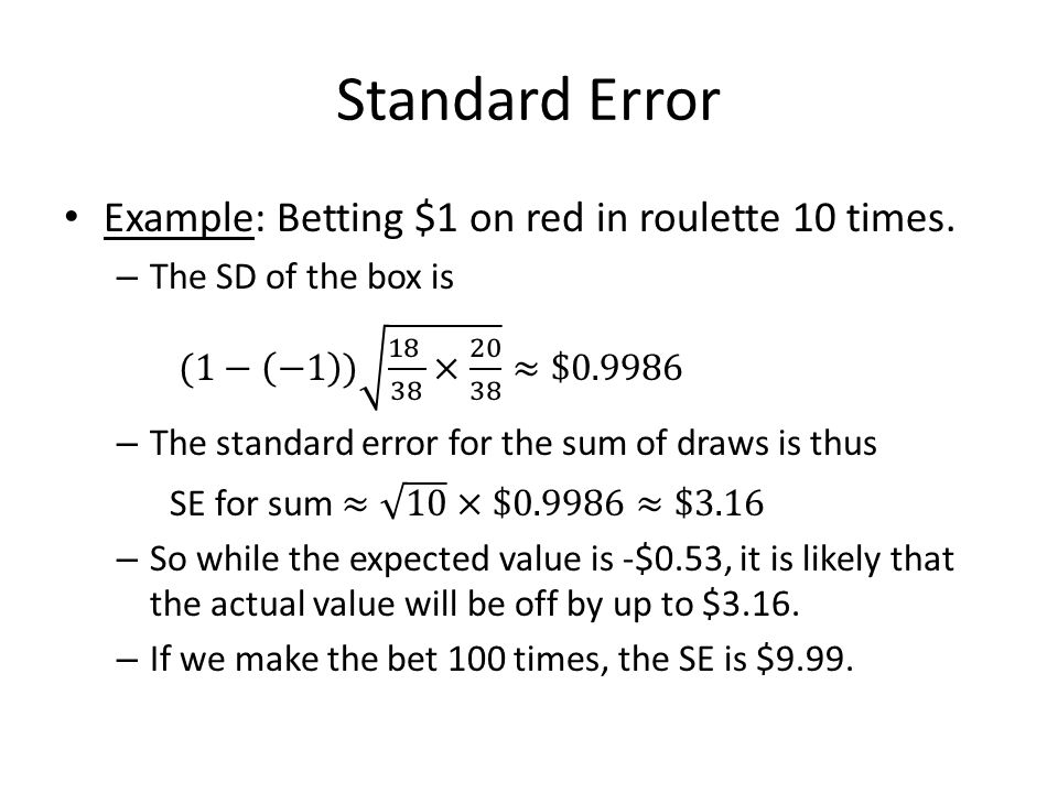
29. Standard Error

33. Activity: Gettysburg Address Choose 10 words at random (or, as randomly as you can) from the Gettysburg Address. Record the mean word length. Choose 20 words at random and record the mean word length (to one decimal place). (Think of this as drawing from a box where tickets are labeled with word lengths.)

34. Probability Histograms And the Central Limit Theorem

35. Probability Histogram A graph representing the probability of each numerical outcome in a chance process. Rectangles have width 1 and are centered on a possible outcome. The area of each rectangle is the probability of the corresponding outcome. Based on chance (theory) not on observations

36. Examples Two dice are rolled and their sum is recorded.

37. Examples Two dice are rolled and their sum is recorded.

38. Examples Two dice are rolled and their sum is recorded. Two dice are rolled and their product is recorded.

39. Probability vs. Density Histogram Example: Roll two dice and record the sum. – Probability histogram

40. Probability vs. Density Histogram Example: Roll two dice and record the sum. – Probability histogram – Repeat the experiment several times and make a density histogram of the results. (http://www.stat.sc.edu/~west/javahtml/CLT.html)http://www.stat.sc.edu/~west/javahtml/CLT.html

41. Probability vs. Density Histogram

42. One hundred random selections of a single word from the Gettysburg Address

43. Normal Approximation A major achievement of 18 th century mathematics was de Moivres proof that the probability histogram for the number of heads in N coin tosses follows the normal curve very closely for large values of N.

44. Central Limit Theorem When drawing at random with replacement from a box, the probability histogram for the sum of the draws or mean of the draws will follow the normal curve, even if the contents of the box do not.

45. Example

46. Central Limit Theorem When drawing at random with replacement from a box, the probability histogram for the sum of the draws or mean of the draws will follow the normal curve, even if the contents of the box do not. – The number of draws must be reasonably large. What reasonably large means does depend on the contents of the box. – To match the normal curve, you must convert to z- values using E.V. and S.E.

47. Central Limit Theorem The probability histogram for the product of the draws will not follow the normal curve.