2. The University of Adelaide, Australia School of Civil, Environmental & Mining Engineering Water Systems and Infrastructure Modelling & Management Group (WaterSIMM) Using Genetic Algorithms to Optimise Network Design and System Operation Including Consideration of Sustainability Professor Angus Simpson Victorian Modelling Group 24 March 2010

3. Outline 1.Simulation of water distribution systems 2.Various formulations of equations 3.Todini and Pilati solution method 4.Genetic algorithm optimisation of water distribution system networks 5.Genetic algorithms for optimising operations of pumping systems 6.Optimising for sustainability

4. My research interests 1.Optimisation of the design and operation of water distribution systems using genetic algorithms [including sustainability considerations (GHGs)] 2.Monitoring health and assessing condition of pipes non-invasively in water distribution systems using small controlled water hammer events

5. My research interests 3.Steady state computer simulation analysis of water distribution systems - improving solvers and modelling of PRVs and FCVs 4.Water hammer modelling in pipelines

6. The research team Total of 14 9 academics (local and overseas) 1 Research Post Doc. 4 PhDs

7. The research team - academics Prof. Angus Simpson Prof. Martin Lambert (condition assessment and genetic algorithms) Prof. Holger Maier (genetic algorithms and sustainability) Dr. Sylvan Elhay – School of Computer Science, The University of Adelaide (steady state solution of pipe networks) Prof. Lang White – School of Electrical and Electronic Engineering, The University of Adelaide (condition assessment)

8. International collaboration Professor Caren Tischendorf – Head of Dept. of Mathematics and Computer Science, University of Cologne, Germany (steady state solution of pipe networks) Dr. Jochen Deuerlein – 3S Consult, Germany (steady state solution of pipe networks, correct modelling of PRVs, FCVs in water networks) – ex-University of Karlsruhe Dr. Arris Tijsseling – University of Eindhoven, The Netherlands (condition assessment) Prof. Wil Schilders – University of Eindhoven, The Netherlands (speeding up solution of nonlinear steady state pipe network equations)

9. Components in a Water Distribution System

10. Simulation of water distribution systems Solution of a set on non-linear equations for –flow (Q) and –pressure (head or hydraulic grade line – H) EPANET uses Todini and Pilati (1987) method – very fast There are many sophisticated commercially available software packages

11. Assumptions Fixed demands – assumed to be not pressure dependent, for example - 100 houses aggregated to a node Various water demand loadings cases –Peak hour (hottest day in summer) –Peak day (extended period simulation usually over 24 hours to check tanks do not run empty) –Fire demand loading cases –Pipe breakage cases

12. Decisions to be made Diameters and locations of pipes Location of pumps Locations and setting of valves (PRVs, FCVs) Locations and elevations of tanks Operation of pumps – off-peak electricity rates Minimising carbon footprint Reliability considerations

13. Design objectives For the economic cost component minimise sum of –Capital cost of the water distribution system (say for a 100 year life) – Present value of pump replacement/refurbishment (every 20 years) –Present value of pump operating costs (100 years)

14. Accounting for Time Present value analysis (PVA) Usually the discount rate i is selected to be cost of capital 6 to 8% For social projects, such as WDSs, a social discount rate should be used, for example, i = 1.4% (intergenerational equity) C: Payment/cost on a given future date t = Number of time periods i = Discount rate

15. Design objectives Satisfy design criteria – for example –Minimum/maximum allowable pressures –Maximum allowable velocities –Tanks must not empty

16. Trial and error approach User has to choose - diameters of pipes, locations of tanks, pumps, and PRVs Engineering judgment and experience Run simulation model for demand load cases Check design criteria and compute cost Adjust sizes of elements in response to pressures Rerun simulation model

17. New York Tunnels problem

18. A very very large search space size Any one of the 21 existing pipes could be duplicated Choose from 16 allowable pipe sizes to meet demands Search space size = 1.43 x 10 21 Eliminate 99.99% of possible solutions by engineering experience (leaves 1.43 x 10 17 )

19. A very very large search space size At 10,000 evaluations per second – can compute 3.15 x 10 11 per year It will take 454,630 years to fully enumerate 0.01% of the total search space (only for 21 decision variables)

20. A typical simple water distribution system

21. Simulation – Solving for The Unknowns Only consider systems with pipes and reservoirs The unknown flow vector (10 pipes in examples) The unknown head vector (7 nodes in example) (gives pressures)

22. A total of 17 unknowns Qs and Hs

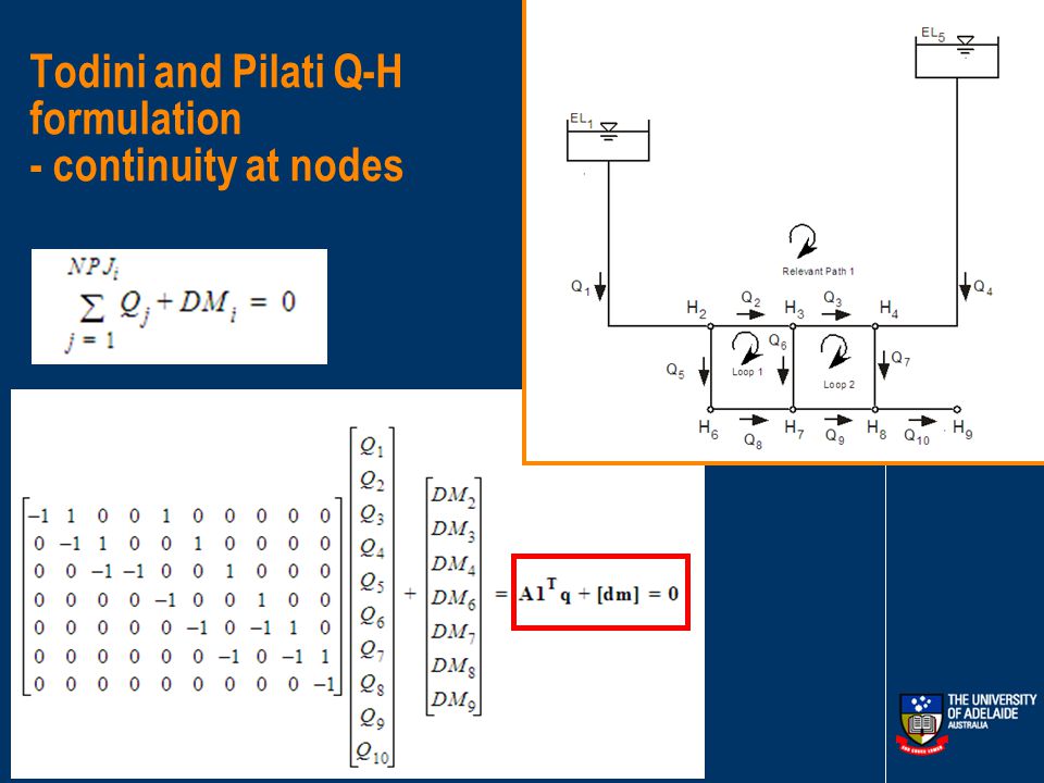
23. Continuity Equation of Flow at a Junction Flow In = Flow Out + Demand (or Withdrawal Discharge) where Q j = flow in pipe j (m 3 /s or ft 3 /s) NPJ i = number of pipes attached to node i DM i = demand at the node i (m 3 /s or ft 3 /s) NJ = total number of nodes in the water distribution system (excluding fixed grade nodes such as reservoirs)

24. Pipe Head Loss Equations in Terms of Nodal Heads where = nodal head at node i in the water distribution system (m or ft) r j = resistance coefficient for the pipe j depending on the head loss relationship (for example, Darcy–Weisbach or Hazen–Williams) Q j = flow in pipe j (m 3 /s or ft 3 /s) n = exponent of the flow in the head loss equation (Darcy–Weisbach n = 2 or Hazen–Williams n = 1.852)

25. Four different non-linear formulations #1 Q-Equations #2 H-Equations #3 LF- Equations (Loop Flow Equations) #4 Todini and Pilati H-Q Equations

26. #1 - The Q-equations formulation (10 unknowns)

27. The Q-equations (10 unknowns)

28. The Q-equations (Newton iterative solution technique)

29. #4 -Todini and Pilati Q-H formulation Define topology matrices Develop block form of equations Use an analytic inverse of block matrices to reduce matrix size from 17 unknowns to 7 unknowns (same as unknown heads H) Fast algorithm

30. Todini and Pilati Q-H formulation Unknowns

31. Todini and Pilati Q-H formulation - Define topology matrices

33. Todini and Pilati Q-H formulation - continuity at nodes

34. Todini and Pilati Q-H formulation – head loss equations for pipes Note that later on the inverse of this matrix will give problems for zero flows

35. Todini and Pilati Q-H formulation – head loss equations for pipes

36. Todini and Pilati Q-H formulation–two sets of equations

37. The Todini and Pilati equations

38. Research Issues Improving solution speed Making solution algorithms more robust – zero flows cause Todini and Pilati method to fail – a regularization method has been developed to control the condition number An improved convergence criterion for stopping has been developed

39. Research Issues Decomposing networks into trees, blocks and bridges to speed up analysis Growing typical networks that have correct mix of loops, links and junctions

40. GENETIC ALGORITHMS FOR OPTIMISATION OF WATER DISTRIBUTION SYSTEMS

41. Types of Evolutionary Algorithms Genetic algorithms (Holland 1976; Goldberg 1989) Ant Colony Optimisation (ACO) Tabu search Simulated annealing Particle swarm optimisation (PSO) Evolutionary strategy (Germany)

42. History of genetic algorithms applied to water distribution systems Pioneered at the University of Adelaide by Laurie Murphy under my supervision in an honours project in 1990 and a PhD starting in 1991 Initial focus was on the optimisation of the design of water distribution systems A spinoff company of Optimatics Pty Ltd formed by University of Adelaide in 1996 – operates in Australia, NZ, USA and UK (employs 20 people) Research focus is now on optimising operations and accounting for multiple objectives (sustainability, reliability)

43. Genetic algorithm optimisation Population orientated technique (select a population size of say 500) Based on mechanisms of natural selection and genetics Selection, crossover and mutation operators produce new generations of designs Fitness of strings drives process Uses EPANET type simulation model to assess performance of all trial water distribution networks in each generation

44. Creating a string from sub-strings - an example BINARY CODING

45. Chromosome of decision variables Choice tables are required for each decision variable Chromosome Existing pipe [3] (binary) 00 = no change, = 2.5 mm 01 = clean/line, = 0.3 mm 10 = duplicate 306 mm 11 = close the pipe

46. Model Operation Optimisation-Simulation Model Link GA OPTIMISATION MODEL HYDRAULIC SIMULATION MODEL Configuration of water distribution and performance passes back and forth

47. Simulate hydraulics of water distribution system Decode each string using the choice tables Run a computer simulation model Simulate demand loading cases consecutively – peak hour, fire, extended period simulation Record any violation of constraints (e.g. pressures too low, velocities too high)

48. Choices for the decision variables

49. Total cost and corresponding fitness of the string Total cost is the: example 1.Real cost of the water distribution system design PLUS 2.A penalty pseudo-cost (or costs) if the constraint(s) are not met – For example =K*Maximum pressure deficit where K=$50,000 per metre Fitness is often taken as the inverse of the total cost

50. Steps in a genetic algorithm optimisation Select a population size (e.g. N=100 or N=500) Select a reproduction or selection operator Select a probability of crossover (P c ) Select a probability of mutation (P m )

51. A Simple Genetic Algorithm This Generation N=500 Selection Crossover & Mutation The Next Generation Mating Pool N=500

52. Tournament selection Randomly select pairs of chromosomes versus Evaluation of the fittest Forming the Mating Pool 11111 11111 1 1 1111 11 1 1 1 11 111 111 1 1 1 1 1 1 111 111 1 1 11 1111111 1111 1 1 11 1 000 0 0 0 00 00 00000 00 000 00000 00000 00000 0 0000 0 00 0 00 0 00 0 1111111000 65 112 94 83 98 143 87 130 Fittest strings win Two sets of tournament selection are required versus FITNESS

53. Crossover (one-point) Chromosome A Chromosome B Parents Chromosome A` Chromosome B ` Offspring 111111 1 111111 1 1 1 111111 1111 000000 00000 00000 000000 Randomly select a crossover point Interchange the tails

54. The mutation operator Mutation occurs with a very small probability One bit switches to a new value

55. Produce many generations Continue to create a series of new generations (say 100,000 different networks) Repeat selection, crossover and mutation Increasingly fit solutions are generated The 10 or so lowest cost solutions must be remembered along the way

56. Designs improve in each generation Best Cost in Each Generation ($ million) 30 40 50 60 70 80 90 100 050,000100,000150,000 200,000 Number of Solution Evaluations New York Tunnels Problem

57. Optimisation of pumping plant operations

58. Murray Bridge – operations optimisation United Utilities – Riverland water treatment plant project at Murray Bridge, South Australia GA optimisation minimises operations electricity costs by –maximizing off-peak pumping and –minimizing static pump head

59. Background Pumps Elevated Storage Water Treatment Plant Clear Water Storage

60. Case study – Murray Bridge system layout White Hill Storage Tank (WHS) Off Takes Murray Bridge Onkaparinga Pipeline Murray Bridge Water Treatment Plant Clear Water Storage Tank (CWS) 3 Parallel Fixed Speed Pumps

61. Traditional approach to control Trigger levels in storage tanks OR Pump scheduling

62. Controls based on trigger levels Lower Trigger Level (Minimum Allowable Level) Upper Trigger Level (Maximum Allowable Level) More Peak Pumping than Necessary Time Tank Level Peak Tariff Period Tank not Full for Next Peak Tariff Period Tank not Full at Start of Peak Tariff Period Off-Peak Tariff Period 7am 9pm

63. Optimisation-Simulation Model Link GA OPTIMISATION MODEL HYDRAULIC SIMULATION MODEL Operating policies for pumping system - trigger levels, schedules for pumps turning on and turning off Model operation

64. Decision variables - operations optimisation at Murray Bridge Used a combination of real-value and integer value representation of the decision variables Four decision variable for final formulation: –Pump start time to fill tank –Pump stop time to drain tank to minimum level –Reduced upper trigger level for tank –Initial level in CWS tank

65. A system controlled with original trigger levels and schedules Lower Trigger Level (Minimum Allowable Level) Upper Trigger Level (Maximum Allowable Level) Time Peak Tariff Period Tank Full at Start of Peak Tariff Period Off-Peak Tariff Period 7am 9pm Start Primary Pump Stop Primary Pump Tank at Minimum Level at End of Peak Tariff Period Tank Level

66. A system controlled with both schedules and a reduced upper trigger level (1) Time Lower Trigger Level (Minimum Allowable Level) Upper Trigger Level (Maximum Allowable Level) Peak Tariff Period Tank Full at Start of Peak Tariff Period Off-Peak Tariff Period 7am 9pm Start Pump Reduced Upper Trigger Level Tank at Minimum Level at End of Peak Tariff Period Tank Level

67. Lower Trigger Level (Minimum Allowable Level) Upper Trigger Level (Maximum Allowable Level) Time Peak Tariff Period Tank Full at Start of Peak Tariff Period Off-Peak Tariff Period 7am 9pm Start Pump Reduced Upper Trigger Level Extended into Off-Peak Tariff Period Tank at Minimum Level at End of Peak Tariff Period Switch Time A system controlled with both schedules and a reduced upper trigger level (2)

68. Modelled System - Original Trigger Levels Level (m) 4 5 6 7 Daily electricity cost (averaged over 28 days) = $313.65 Time (hrs) Daily peak pumping (averaged over 28 days): $286.05 Initial Level in CWS = 3.4m Lower trigger level = 5.49m Upper trigger level = 6.98m 0 1 2 3 8 11 am9 am7 am 5 am3 am1 am11 pm9 pm7 pm5 pm3 pm1 pm Daily off-peak pumping (averaged over 28 days): $27.60 WHS (m) CWS (m) WHS and CWS tank levels for first 24 hours of a 28-day simulation under fixed trigger level control for a 7.17 ML/D flow

69. Optimised system - new approach Initial Level in CWS = 3.675 m Lower trigger level = 5.49 m Reduced trigger level = 5.76 m Upper trigger level = 6.98m WHS and CWS tank levels after optimisation for a 7.17 ML/D flow 0 1 2 3 4 5 6 7 8 Time (hrs) Level (m) WHS CWS Pump on at 1:54:13 am Peak Pumping: $189.51 Off-peak Pumping: $67.63 Total electricity cost = $257.14. Hence a $56.51 or 18.0% 11 am9 am7 am 5 am3 am1 am11 pm9 pm7 pm5 pm3 pm 1 pm Switch time 2:15 am

70. Results - savings from new approach 18.284.34378.76463.110 13.646.3293.02339.328 18.056.48257.16313.647.17 22.459.72207.13266.866 22.936.17121.57157.744 54.950.6141.6592.262 (%)($) Improved Controls Current Controls Savings Pumping Cost ($/Day) Daily Demand (ML/Day)

71. Accounting for Sustainability in the Design and Operation of Water Distribution Pumping Systems

72. Design and Optimisation of Water Distribution Systems (WDSs) –Traditional considerations: System capital and operating costs of WDSs –New considerations: GHG emissions of WDSs –Aim to minimise economic costs on a total life cycle basis –Aim to minimise GHG emissions on a total life cycle basis –These two objectives conflict and cannot be satisfied simultaneously

73. Research Objectives To construct a sustainability integrated multi-objective genetic algorithm optimisation model for the planning, design and evaluation of WDSs To explore the impacts different sustainability criteria (Greenhouse Gas emissions) will have on the results of WDS optimisation

74. Aspects of Sustainability - Social Environmental Economic Technical 1: Total cost of the system 2: GHG emissions 3:Systemreliability 4: Robustness of Pareto-optimal Front

75. Two of the Main Conflicting Objectives Minimisation of the total life cycle system costs Minimisation of the total life cycle system GHG emissions

76. Higher Cost Lower GHG Lower Cost Higher GHG Big pump Small pipe Small pump Big pipe

77. Evaluating multi-objective optimisation results using a Pareto tradeoff curve Cost GHG Tradeoff Curve

78. Determining life cycle economic costs Total Cost Capital Costs Pipes and Pump Stations Pump Refurbishment Costs (PVA) Pumps Operating Costs (PVA) Pumping

79. Determining life cycle GHG emissions (no discounting i = 0% IPCC) Emission Factor Analysis

80. Optimisation Framework Generate Options MOGA Simulation Evaluation Comparison & Selection WDS Optimisation Objectives Minimisation of total cost Minimisation of GHG emissions Maximisation of system reliability Maximisation of robustness of Pareto- optimal solutions

81. Multi-objective optimisation using genetic algorithms MOGA: NSGA-II Generate initial population Objective evaluation Simulation models Ranking Generate global population Non-dominated sorting Crowding distance Comparison & selection Constraint handling Generate child population Crossover Mutation Stopping criteria met? Stop Yes No

82. Case Study The network consists of a lower reservoir (water source), one pump, one rising main and an upper reservoir

83. Case Study The aim –to select the best combination of the pump size and pipe size –deliver the minimum average peak-day flow –minimise both the total cost and GHG emissions of the network during its design life

84. Pareto optimal tradeoff curve – multi-objective optimisation i = 6% Diameter for lowest cost solution

85. Tradeoff for i = 1.4% Lowest cost Lowest GHGs

86. Conclusions Evolutionary algorithm optimisation has application in design and operation of water distribution systems It is relatively easy to tack on an evolutionary algorithm optimisation onto existing simulation models Capital costs and operating costs can be reduced significantly Sustainability can be optimised