1. CE-632 Foundation Analysis and Design
Instructor:
Dr. Amit Prashant, FB 304, PH#

2. Reference Books

3. Grading Policy Two 60-min Mid Semester Exams ……. 30%
End Semester Exam …………… %
Assignment ……………………………… 10%
Projects/ Term Paper -…………………… 20%
TOTAL %
Course Website:

4. Soil Mechanics Review Soil behavour is complex:
Anisotropic
Non-homogeneous
Non-linear
Stress and stress history dependant
Complexity gives rise to importance of:
Theory
Lab tests
Field tests
Empirical relations
Computer applications
Experience, Judgement, FOS

5. Soil Texture Particle size, shape and size distribution
Coarse-textured (Gravel, Sand)
Fine-textured (Silt, Clay)
Visibility by the naked eye (0.05mm is the approx limit)
Particle size distribution
Sieve/Mechanical analysis or Gradation Test
Hydrometer analysis for smaller than .05 to .075 mm (#200 US Standard sieve)
Particle size distribution curves
Well graded
Poorly graded

6. Effect of Particle size

7. Basic Volume/Mass Relationships

8. Additional Phase Relationships
Typical Values of Parameters:

9. Atterberg Limits
Liquid limit (LL): the water content, in percent, at which the soil changes from a liquid to a plastic state.
Plastic limit (PL): the water content, in percent, at which the soil changes from a plastic to a semisolid state.
Shrinkage limit (SL): the water content, in percent, at which the soil changes from a semisolid to a solid state.
Plasticity index (PI): the difference between the liquid limit and plastic limit of a soil, PI = LL – PL.

10. Clay Mineralogy Clay fraction, clay size particles
Particle size < 2 µm (.002 mm)
Clay minerals
Kaolinite, Illite, Montmorillonite (Smectite)
- negatively charged, large surface areas
Non-clay minerals
- e.g. finely ground quartz, feldspar or mica of "clay" size
Implication of the clay particle surface being negatively charged double layer
Exchangeable ions
- Li+<Na+<H+<K+<NH4+<<Mg++<Ca++<<Al+++
- Valance, Size of Hydrated cation, Concentration
Thickness of double layer decreases when replaced by higher valence cation - higher potential to have flocculated structure
When double layer is larger swelling and shrinking potential is larger

11. Clay Mineralogy
Soils containing clay minerals tend to be cohesive and plastic.
Given the existence of a double layer, clay minerals have an affinity for water and hence has a potential for swelling (e.g. during wet season) and shrinking (e.g. during dry season). Smectites such as Montmorillonite have the highest potential, Kaolinite has the lowest.
Generally, a flocculated soil has higher strength, lower compressibility and higher permeability compared to a non-flocculated soil.
Sands and gravels (cohesionless ) : Relative density can be used to compare the same soil. However, the fabric may be different for a given relative density and hence the behaviour.

12. Soil Classification Systems
Classification may be based on – grain size, genesis, Atterberg Limits, behaviour, etc. In Engineering, descriptive or behaviour based classification is more useful than genetic classification.
American Assoc of State Highway & Transportation Officials (AASHTO)
Originally proposed in 1945
Classification system based on eight major groups (A-1 to A-8) and a group index
Based on grain size distribution, liquid limit and plasticity indices
Mainly used for highway subgrades in USA
Unified Soil Classification System (UCS)
Originally proposed in 1942 by A. Casagrande
Classification system pursuant to ASTM Designation D-2487
Classification system based on group symbols and group names
The USCS is used in most geotechnical work in Canada

13. Soil Classification Systems
Group symbols: G - gravel S - sand M - silt C - clay O - organic silts and clay Pt - peat and highly organic soils H - high plasticity L - low plasticity W - well graded P - poorly graded
Group names: several descriptions
Plasticity Chart

14. Grain Size Distribution Curve
Gravel:
Sand:

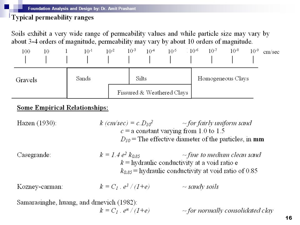
15. Permeability
Flow through soils affect several material properties such as shear strength and compressibility
If there were no water in soil, there would be no geotechnical engineering Darcy’s Law
Developed in 1856
Unit flow,
Where: K = hydraulic conductivity
∆h =difference in piezometric or “total” head
∆L = length along the drainage path
Definition of Darcy’s Law
Darcy’s law is valid for laminar flow Reynolds Number: Re < 1 for ground water flow

17. Permeability of Stratified Soil

18. Seepage 1-D Seepage: Q = k i A 2-D Seepage (flow nets)
where, i = hydraulic gradient =∆h /∆L
∆h = change in TOTAL head
Downward seepage increases effective stress
Upward seepage decreases effective stress
2-D Seepage (flow nets)

19. Effective Stress
Effective stress is defined as the effective pressure that occurs at a specific point within a soil profile
The total stress is carried partially by the pore water and partially by the soil solids, the effective stress, σ’, is defined as the total stress, σt, minus the pore water pressure, u, σ' = σ − u

20. Effective Stress
Changes in effective stress is responsible for volume change
The effective stress is responsible for producing frictional resistance between the soil solids
Therefore, effective stress is an important concept in geotechnical engineering
Overconsolidation ratio, Where: σ´c = preconsolidation pressure
Critical hydraulic gradient σ′ = 0 when i = (γb-γw) /γw → σ′ = 0

21. Effective Stress Profile in Soil Deposit

22. Example
Determine the effective stress distribution with depth if the head in the gravel layer is a) 2 m below ground surface b) 4 m below ground surface; and c) at the ground surface.
Steps in solving seepage and effective stress problems:
set a datum
evaluate distribution of total head with depth
subtract elevation head from total head to yield pressure head
calculate distribution with depth of vertical “total stress”
subtract pore pressure (=pressure head x γw) from total stress

23. Vertical Stress Increase with Depth
Allowable settlement, usually set by building codes, may control the allowable bearing capacity
The vertical stress increase with depth must be determined to calculate the amount of settlement that a foundation may undergo
Stress due to a Point Load
In 1885, Boussinesq developed a mathematical relationship for vertical stress increase with depth inside a homogenous, elastic and isotropic material from point loads as follows:

24. Vertical Stress Increase with Depth
For the previous solution, material properties such as Poisson’s ratio and modulus of elasticity do not influence the stress increase with depth, i.e. stress increase with depth is a function of geometry only.
Boussinesq’s Solution for point load-

25. Stress due to a Circular Load
The Boussinesq Equation as stated above may be used to derive a relationship for stress increase below the center of the footing from a flexible circular loaded area:

26. Stress due to a Circular Load

27. Stress due to Rectangular Load
The Boussinesq Equation may also be used to derive a relationship for stress increase below the corner of the footing from a flexible rectangular loaded area:
Concept of superposition may also be employed to find the stresses at various locations.

28. Newmark’s Influence Chart
The Newmark’s Influence Chart method consists of concentric circles drawn to scale, each square contributes a fraction of the stress
In most charts each square contributes 1/200 (or 0.005) units of stress (influence value, IV)
Follow the 5 steps to determine the stress increase:
Determine the depth, z, where you wish to calculate the stress increase
Adopt a scale of z=AB
Draw the footing to scale and place the point of interest over the center of the chart
Count the number of elements that fall inside the footing, N
Calculate the stress increase as:

29. Simplified Methods
The 2:1 method is an approximate method of calculating the apparent “dissipation” of stress with depth by averaging the stress increment onto an increasingly bigger loaded area based on 2V:1H.
This method assumes that the stress increment is constant across the area (B+z)·(L+z) and equals zero outside this area.
The method employs simple geometry of an increase in stress proportional to a slope of 2 vertical to 1 horizontal
According to the method, the increase in stress is calculated as follows:

30. Consolidation Settlement – total amount of settlement
Consolidation – time dependent settlement
Consolidation occurs during the drainage of pore water caused by excess pore water pressure

31. Settlement Calculations
Settlement is calculated using the change in void ratio

32. Settlement Calculations

33. Example

34. Consolidation Calculations
Consolidation is calculated using Terzaghi’s one dimensional consolidation theory
Need to determine the rate of dissipation of excess pore water pressures

35. Consolidation Calculations

36. Example

37. Shear Strength Soil strength is measured in terms of shear resistance
Shear resistance is developed on the soil particle contacts
Failure occurs in a material when the normal stress and the shear stress reach some limiting combination

38. Direct shear test
Simple, inexpensive, limited configurations

39. Triaxial Test Consolidated Drained Test
may be complex, expensive, several configurations
Consolidated Drained Test

40. Triaxial Test Undrained Loading (f = 0 Concept)
Total stress change is the same as the pore water pressure increase in undrained loading, i.e. no change in effective stress
Changes in total stress do not change the shear strength in undrained loading

41. Stress-Strain Relationships

42. Failure Envelope for Clays

43. Unconfined Compression Test
A special type of unconsolidated-undrained triaxial test in which the confining pressure, σ3, is set to zero
The axial stress at failure is referred to the unconfined compressive strength, qu (not to be confused with qu)
The unconfined shear strength, cu, may be defined as,

44. Stress Path

45. Elastic Properties of Soil

46. Elastic Properties of Soil

47. Hyperbolic Model
Empirical Correlations for cohesive soils

48. Anisotropic Soil Masses
Generalized Hook’s Law for cross-anisotropic material
Five elastic parameters