1. The Best-First Search Algorithm
Implementing Best-First Search
In spite of their limitations, algorithms such as backtrack, hill climbing, and dynamic programming can be used effectively if their evaluation functions are sufficiently informative to avoid local maxima, dead ends, and related anomalies in a search space. In general, however, use or heuristic search requires a more flexible algorithm: this is provided by best-first search, where, with a priority queue, recovery from these situations is possible. Like the depth-first and breadth-first search algorithms or Chapter 3, best-first search uses lists to maintain states: open to keep track or the current fringe of the search and closed to record states already visited. An added step in the algorithm orders the states on open according to some heuristic estimate or their "closeness" to a goal. Thus, each iteration or the loop considers the most "promising" state on the open list. The pseudo code for the function best-first search appears below.

2. begin
open := [Start]; % initialize
closed :=[];
while open ≠ [] do % states remain
remove the leftmost state from open, call it X;
if X = goal then return the path from Start to X
else begin
generate children of X;
for each child of X do
case
the child is not on open or closed:
assign the child a heuristic value;
add the child to open
end;
the child is already on open:
if the child was reached by a shorter path
then give the state on open the shorter path
the child is already on closed:
if the child was reached by a shorter path then
remove the state from closed;
end; % case
put X on closed;
re-order states on open by heuristic merit (best leftmost)
return FAIL % open is empty
end.

3. At each iteration, best_first_search removes the first element from the open list. If it meets the goal conditions, the algorithm returns the solution path that led to the goal. Note that each state retains ancestor information to determine if it had previously been reached by a shorter path and to allow the algorithm to return the final solution path. (See Section )
If the first element on open is not a goal, the algorithm applies all matching production rules or operators to generate its descendants. If a child state is already on open or closed, the algorithm checks to make sure that the state records the shorter of the two partial solution paths. Duplicate states are not retained. By updating the ancestor history of nodes on open and closed when they are rediscovered, the algorithm is more likely to find a shorter path to a goal.
best_first_search then applies a heuristic evaluation to the states on open, and the list is sorted according to the heuristic values of those states. This brings the "best" states to the front of open. Note that because these estimates are heuristic in nature, the next state to be examined may be from any level of the state space. When open is maintained as a sorted list, it is often referred to as a priority queue.
Figure 4.10 shows a hypothetical state space with heuristic evaluations attached to some of its states. The states with attached evaluations arc those actually generated in best_first_search. The states expanded by the heuristic search algorithm are indicated in bold; note that it does not search all of the space. The goal of best-first search is to find the goal state by looking at as few states as possible; the more informed (Section 4.2.3) the heuristic, the fewer states arc processed in finding the goal.
A trace of the execution of best_first_search on this graph appears below. Suppose P is the goal state in the graph of Figure Because P is the goal, states along the path to P tend to have low heuristic values. The heuristic is fallible: the state 0 has a lower value than the goal itself and is examined first. Unlike hill climbing, which does not maintain a priority queue for the selection of "next" states, the algorithm recovers from this error and finds the correct goal.

6. 1. open = [A5]; closed = []
2. evaluate A5; open = [B4,C4,D6]; closed = [A5]
3. evaluate B4; open = [C4,E5.F5,D6]; closed = [B4,A5]
4. evaluate C4; open = [H3,G4,ES,F5,D6]; closed = [C4,B4,A5]
5. evaluate H3; open = [O2,P3,G4,E5,F5,D6]; closed = [H3,C4,B4,A5]
6. evaluate o2; open = [P3,G4,E5,F5,D6]; closed = [O2,H3,C4,B4,A5)
7. evaluate P3; the solution is found!
Figure 4,11 shows the space as it appears after the fifth iteration of the while loop. The states contained in open and closed are indicated. open records the current frontier of the search and closed records states already considered. Note that the frontier of the search is highly uneven, reflecting the opportunistic nature of best-first search.
The best-first search algorithm always selects the most promising state on open for further expansion. However, as it is using a heuristic that may prove erroneous, it does not abandon all the other states but maintains them on open. In the event a heuristic Ieads the search down a path that proves incorrect, the algorithm will eventually retrieve some previously generated, "next best" state from open and shift its focus to another part of the space. In the example of Figure 4.10, after the children of state B were found to have poor heuristic evaluations, the search shifted its focus to state C. The children of B were kept on open in case the algorithm needed to return to them later. In best_first_search, as in the algorithms of Chapter 3, the open list allows backtracking from paths that fail to produce a goal.
We now evaluate the performance of several different heuristics for solving the 8-puzzle. Figure 4.12 shows a start and goal state for the 8-puzzle, along with the first three states generated in the search.
The simplest heuristic counts the tiles out of place in each state when it is compared with the goal. This is intuitively appealing, because It would seem that, all else being equal, the state that had fewest tiles out of place is probably closer to the desired goal and would be the best to examine next.
However, this heuristic does not use all of the information available in a board configuration, because it does not take into account the distance the tiles must be moved.

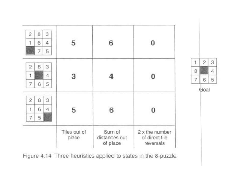
8. A "better“ heuristic would sum all the distances by which the tiles are out of place, one for each square a tile must be moved to reach its position in the goal state.
Both of these heuristics can be criticized for failing to acknowledge the difficult of tile reversals. That is, if two tiles are next to each other and the goal requires their being in opposite locations, it takes (many) more than two moves to put them back in place, as the tiles must "go around" each other (Figure 4.13).
A heuristic that takes this into account multiplies a small number (2, for example) times each direct tile reversal (where two adjacent tiles must be exchanged to be in the order of the goal). Figure 4.14 shows the result of applying each of these three heuristics to the three child states of Figure 4.12.
In Figure 4.14's summary of evaluation functions, the “sum of distances” heuristic does indeed seem to provide a more accurate estimate of the work to be done than the simple count of the number of tiles out of place. Also, the tile reversal heuristic fails to distinguish between these states, giving each an evaluation of 0. Although it is an intuitively appealing heuristic, it breaks down since none of these states have any direct reversals. A fourth heuristic, which may overcome the limitations of the tile reversal heuristic, adds the sum of the distances the tiles are out of place and 2 times the number of direct reversals.

10. This example illustrates the difficulty of devising good heuristics
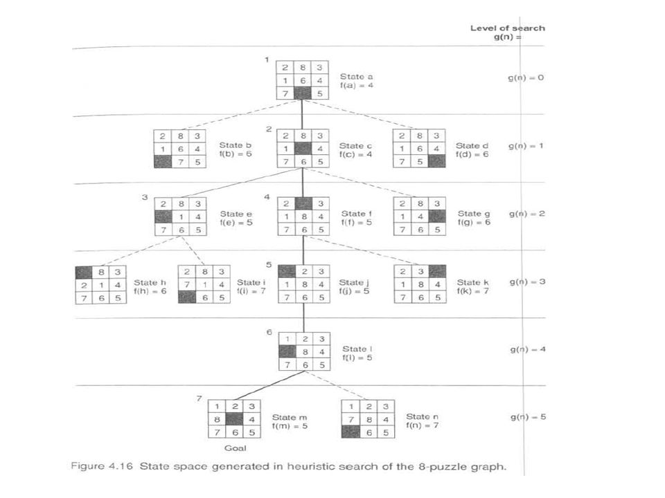
This example illustrates the difficulty of devising good heuristics. Our goal is to use the limited information available in a single state descriptor to make intelligent choices. Each of the heuristics proposed above ignores some critical bit of information and is subject to improvement. The design of good heuristics is an empirical problem; judgment and intuition help, but the final measure of a heuristic must be its actual performance on problem instances.
Because heuristics are fallible, it is possible that a search algorithm can be misled down some path that fails to lead to a goal. This problem arose in depth-first search, where a depth count was used to detect fruitless paths. This idea may also be applied to heuristic search. If two states have the same or nearly the same heuristic evaluations, it is generally preferable to examine the state that is nearest to the root state of the graph. This state will have a greater probability of being on the shortest path to the goal. The distance from the starting state to its descendants can be measured by maintaining a depth count for each state. This count is 0 for the beginning state and is incremented by 1 for each level of the search. It records the actual number of moves that have been used to go from the starting state in the search to each descendant. This depth measure can be added to the heuristic evaluation of each state to bias search m favor of states found shallower in the graph.
This makes our evaluation function, f, the sum of two components:
f(n) = g(n) + h(n)
where g(n) measures the actual length of the path from any state n to the start state and h(n) is a heuristic estimate of the distance from state n to a goal.
In the 8-puzzlc, for example, we can let h(n) be the number of tiles out of place. When
this evaluation is applied to each of the child states in Figure 4.12, their f values are 6, 4, and 6, respectively, see Figure 4.15.
The full best-first search of the 8-puzzlc graph, using f as defined above, appears in Figure Each state is labeled with a letter and its heuristic weight, f(n) = g(n) + h(n). The number at the top of each state indicates the order in which it was taken off the open list. Some states (h, g, b, d, n, k, and i) are not so numbered, because they were still on open when the algorithm terminated.

11. The successive stages of open and closed that generate this graph are:
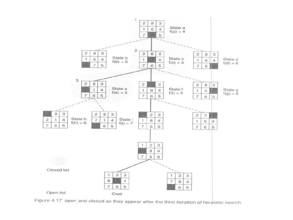
2. open = [ c4, b6, d6];
closed = [a4]
3. open = [e5, f5, b6, d6, g6];
closed = [a4, c4]
4. open = [ f5, h6, b6, d6, g6, l7];
closed = [a4, c4, e5]
5. open = [ j5, h6, b6, d6, g6, k7, l7];
closed = [a4, c4, e5, f5]
6. open = [ l5, h6, b6, d6, g6, k7, l7];
closed = [ a4, c4, e5, f5, j5]
7. open = [ m5, h6, b6, d6, g6, n7, k7, l7]:
closed = [a4, c4, e5, f5, j5, l5]
8. success, m = goal!
In step 3, both e and f have a heuristic of 5. State e is examined first, producing children, h and i. Although h, the child of e, has the same number of tiles out of place as f, it is one level deeper in the space. The depth measure, g(n), causes the algorithm to select f for evaluation in step 4. The algorithm goes back to the shallower state and continues to the goal. The state space graph at this stage of the search, with open and closed highlighted, appears in Figure Notice the opportunistic nature of best-first search.

13. In effect, the g(n) component of the evaluation function gives the search more of a breadth-first flavor. This prevents it from being misled by an erroneous evaluation: if a heuristic continuously returns “good” evaluations for states along a path that fails to reach a goal, the g value will grow to dominate h and force search back to a shorter solution path. This guarantees that the algorithm will not become permanently lost, descending an infinite branch. Section 4.2 examines the conditions under which best-first search using this evaluation function can actually be guaranteed to produce the shortest path to a goal.
To summarize:
I. Operations on states generate children of the state currently under examination.
2. Each new state is checked to see whether it has occurred before (is on either open or closed), thereby preventing loops.
3. Each state n is given an f value equal to the sum of its depth in the search space g(n) and a heuristic estimate of its distance to a goal h(n). The h value guides search toward heuristically promising states while the g value prevents search from persisting indefinitely on a fruitless path.
4. States on open are sorted by their f values. By keeping all states on open until they are examined or a goal is found, the algorithm recovers from dead ends.
5. As an implementation point, the algorithm's efficiency can be improved through maintenance of the open and closed lists, perhaps as heaps or leftist trees.
Best-first search is a general algorithm for heuristically searching any state space graph (as were the breadth- and depth-first algorithms presented earlier). It is equally applicable to data- and goal-driven searches and supports a variety of heuristic evaluation functions. It will continue (Section 4.2) to provide a basis for examining the behavior of heuristic search. Because of its generality, best-first search can be used with a variety of heuristics, ranging from subjective estimates a state's "goodness" to sophisticated measures based on the probability of a state leading to a goal. Bayesian statistical measures (Chapter 7) offer an important example of this approach.

15. Another interesting approach to implementation heuristics is the use of confidence measures by expert systems to weigh the results of a rule. When human experts employ a heuristic, they are usually able to give some estimate of their confidence in its conclusions. Expert systems employ confidence measures to select the conclusions with the highest likelihood of success. States with extremely low confidence can be eliminated entirely . This approach to heuristic search is examined in the next section.
Heuristic Search and Expert Systems
Simple games such as the 8-puzzle are ideal vehicles for exploring the design and behavior of heuristic search algorithms for a number of reasons:
1. The search spaces are large enough to require heuristic pruning.
2. Most games are complex enough to suggest a rich variety of heuristic evaluations for comparison and analysis.
3. Games generally do not involve complex representational issues. A single node of the state space is just a board description and usually can be captured in a straightforward fashion. This allows researchers to focus on the behavior of the heuristic, rather than the problems of knowledge representation.
4. Because each node of the state space has a common representation (e.g., a board description), a single heuristic may be applied throughout the search space. This contrasts with systems such as the financial advisor, where each node represents a different subgoal with its own distinct description.
More realistic problems greatly complicate the implementation and analysis of heuristic search by requiring multiple heuristics to deal with different situations in the problem space. However, the insights gained from simple games generalize to problem such as those found in expert systems applications, planning, intelligent control , and machine learning. Unlike the 8-puzzle, a single heuristic may not apply to each state in these domains.

16. Instead, situation specific problem-solving heuristics are encoded in the syntax and content of individual problem solving operators. Each solution step incorporates its own heuristic that determines when it should be applied; the pattern matcher matches the appropriate operation (heuristic) with the relevant state in the space.
THE FINANCIAL ADVISOR, REVISITED
The use of heuristic measures to guide search is a general approach in AI. Consider again the financial advisor problem of Chapters 2 and 3, where the knowledge base was treated as a set of logical implications, whose conclusions are either true or false. In actuality, these rules are highly heuristic in nature. For example, one rule states that an individual with adequate savings and income should invest in stocks:
savings_account(adequate) ^ income(adequate)  investment(stocks).
In reality, it is possible that such an individual may prefer the added security of a combination strategy or even that of placing all investment money in savings. Thus, the rule is a heuristic, and the problem solver should try to account for this uncertainty. We could take additional factors, such as the age of the investor and the long-term prospects for security and advancement in the investor's profession, into account to make the rules more informed and capable of finer distinctions. However, this does hot change the fundamentally heuristic nature of financial advice.
One way in which expert systems have addressed this issue is to attach a numeric weight (called a confidence measure or certainty factor) to the conclusion of each rule. This measures the confidence that may be placed in their conclusions.
Each rule conclusion is given a confidence measure, a real number between -1 and 1, with 1 corresponding to certainty (true) and -1 to a definite value or false. Values in between reflect varying confidence in the conclusion. For example, the preceding rule may be given a confidence of, say, 0.8, reflecting a small possibility that it may not be correct. Other conclusions may be drawn with different confidence weights:

17. savings_account(adequate) ^ income(adequate)  investment(stocks)
with confidence = 0.8.
savings_account(adequate) ^ income(adequate)  investment(combination)
with confidence = 0.5.
savings_account(adequate) ^ income(adequate)  investment(savings)
with confidence = 0.1.
These rules reflect the common investment advice that although an individual with adequate savings and income would be most strongly advised to invest in stocks, there is some possibility that a combination strategy should be pursued and a slight chance that they may want to continue investing in savings. Heuristic search algorithms can use these certainty factors in a number of ways. For example, the results of all applicable rules could be produced along with their associated confidences. This exhaustive search of all possibilities may be appropriate in domains such as medicine. Alternatively, the program might return only the result with the strongest confidence value, if alternative solutions are not of interest. This can allow the program to ignore other rules, radically pruning the search space. A more conservative pruning strategy could ignore rules that draw a conclusion with a confidence less than a certain value, 0.2 for example.
A number of important issues must be addressed in using confidence measures to weight rule conclusions. What does it really mean to have a "numeric confidence measure"? For example, how are the confidences handled if the conclusion of one rule is used as the premise of others? How are confidences combined in the event that more than one rule draws the same conclusion? How are the proper confidence measures assigned to rules in the first place? These issues are discussed in more detail in Chapter 7.