1. Desired Bode plot shape Ess requirement Noise requirement 0 -90 -180 0dB gcd High low-freq-gain for steady state tracking Low high-freq-gain for noise attenuation Sufficient PM near gc for stability PM d Mid frequency

2. Desired Bode plot shape 0 -90 -180 0dB gc High low freq gain for steady state tracking Low high freq gain for noise attenuation Sufficient PM near gc for stability Low freq High freq Want high gain Want low gain Mid freq Want sufficient Phase margin Use low pass filters Use PI or lag control Use lead or PD control PM+Mp=70

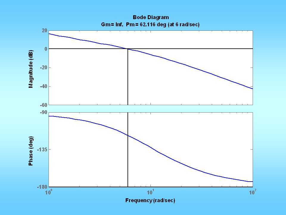
3. C(s)G p (s) Controller design with Bode From specs: => desired Bode shape of G ol (s) Make Bode plot of G p (s) Add C(s) to change Bode shape Get closed loop system Run step response, or sinusoidal response

4. Mr and BW are widely used Closed-loop phase resp. rarely used

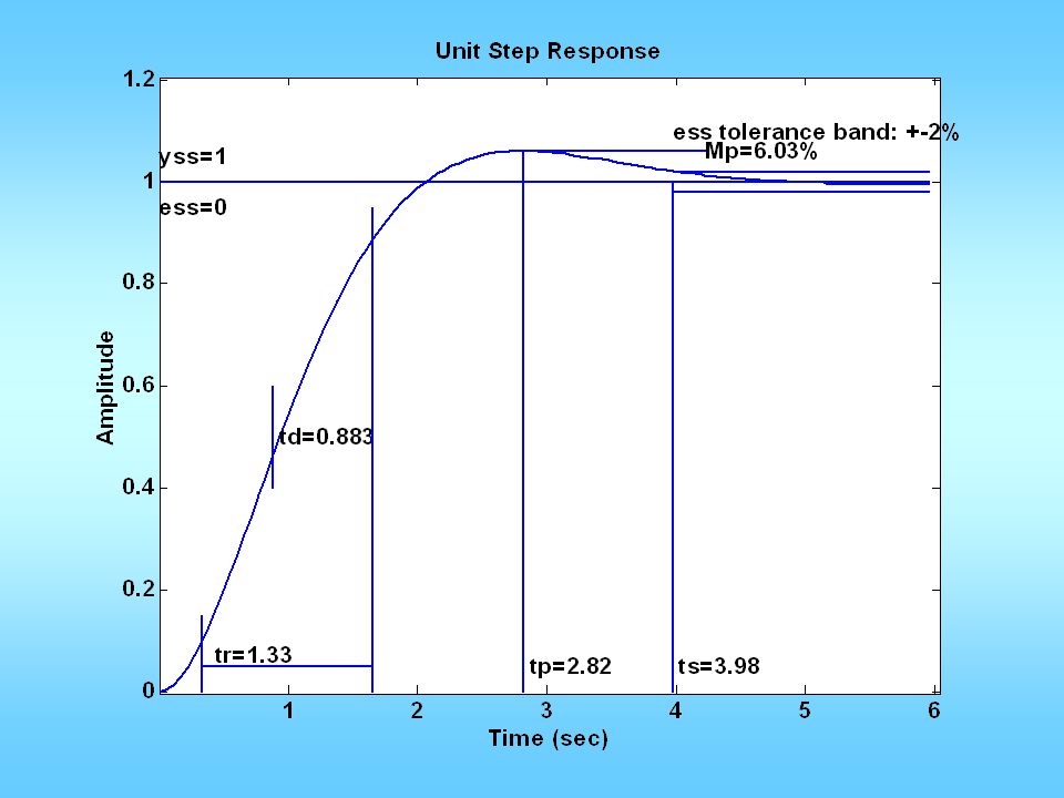
5. Important relationships Closed-loop BW are very close to n Open-loop gain cross over gc (0.65~0.8)* n, When <= 0.6, r and n are close When >= 0.7, no resonance determines phase margin and Mp: 0.40.50.60.7 PM44536167deg 100 Mp2516105% PM+Mp 70

6. Mid frequency requirements gc is critically important –It is approximately equal to closed-loop BW –It is approximately equal to n Hence it determines tr, td directly PM at gc controls –Mp 70 – PM PM and gc together controls and d –Determines ts, tp Need gc at the right frequency, and need sufficient PM at gc

7. Low frequency requirements Low freq gain slope and/or phase determines system type Height of at low frequency determine error constants Kp, Kv, Ka Which in turn determine ess Need low frequency gain plot to have sufficient slope and sufficient height

8. High frequency requirements Noise is always present in any system Noise is rich in high frequency contents To have better noise immunity, high frequency gain of system must be low Need loop gain plot to have sufficient slope and sufficiently small value at high frequency

9. Overall Loop shaping strategy Determine mid freq requirements –Speed/bandwidth gc –Overshoot/resonance PM d Use PD or lead to achieve PM d @ gc Use overall gain K to enforce gc PI or lag to improve steady state tracking –Use PI if type increase neede –Use lag if ess needs to be reduced Use low pass filter to reduce high freq gain

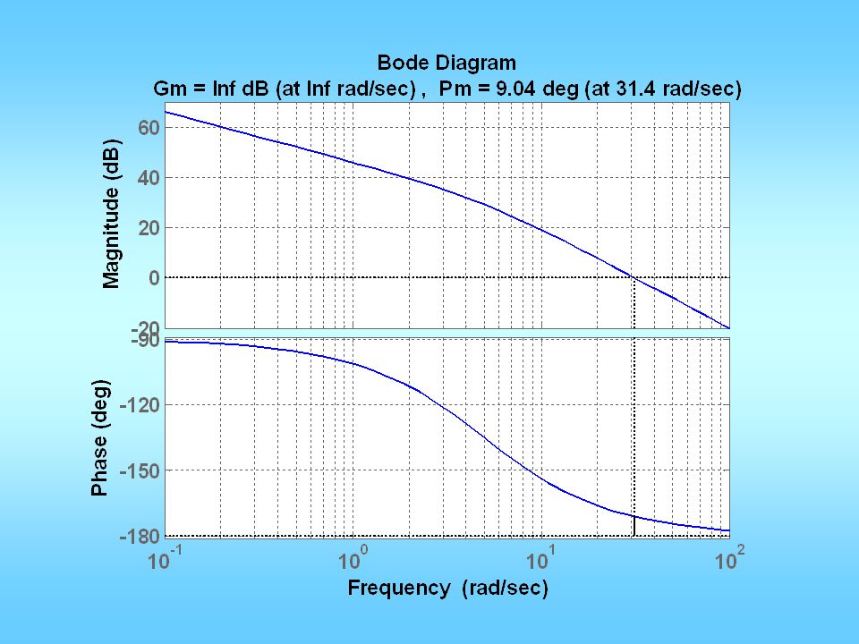
10. Proportional controller design Obtain open loop Bode plot Convert design specs into Bode plot req. Select K P based on requirements: –For improving ess: K P = K p,v,a,des / K p,v,a,act –For fixing Mp: select gcd to be the freq at which PM is sufficient, and K P = 1/|G(j gcd )| –For fixing speed: from td, tr, tp, or ts requirement, find out n, let gcd = (0.65~0.8)* n and K P = 1/|G(j gcd )|

11. clear all; n=[0 0 40]; d=[1 2 0]; figure(1); clf; margin(n,d); %proportional control design: figure(1); hold on; grid; V=axis; Mp = 10; %overshoot in percentage PMd = 70-Mp + 3; semilogx(V(1:2), [PMd-180 PMd-180],':r'); %get desired w_gc x=ginput(1); w_gcd = x(1); KP = 1/abs(evalfr(tf(n,d),j*w_gcd)); figure(2); margin(KP*n,d); figure(3); mystep(KP*n, d+KP*n);

16. PD Controller

17. 20*log(KP) KP/KD Place gcd here Bad for noise

18. PD control design

19. n=[0 0 1]; d=[0.02 0.3 1 0]; figure(1); clf; margin(n,d); Mp = 10/100; zeta = sqrt((log(Mp))^2/(pi^2+(log(Mp))^2)); PMd = zeta * 100 + 3; tr = 0.3; w_n=1.8/tr; w_gcd = w_n; PM = angle(polyval(n,j*w_gcd)/polyval(d,j*w_gcd)); phi = PMd*pi/180-PM; Td = tan(phi)/w_gcd; KP = 1/abs(polyval(n,j*w_gcd)/polyval(d,j*w_gcd)); KP = KP/sqrt(1+Td^2*w_gcd^2); KD=KP*Td; ngc = conv(n, [KD KP]); figure(2); margin(ngc,d); figure(3); mystep(ngc, d+ngc); Could be a little less

20. PD control design Variation Restricted to using K P = 1 Meet M p requirement Find gc and PM Find PM d Let = PMd – PM + (a few degrees) Compute T D = tan( )/w gcd K P = 1; K D =K P T D

21. n=[0 0 5]; d=[0.02 0.3 1 0]; figure(1); clf; margin(n,d); Mp = 10/100; zeta = sqrt((log(Mp))^2/(pi^2+(log(Mp))^2)); PMd = zeta * 100 + 18; [GM,PM,wgc,wpc]=margin(n,d); phi = (PMd-PM)*pi/180; Td = tan(phi)/wgc; Kp=1; Kd=Kp*Td; ngc = conv(n, [Kd Kp]); figure(2); margin(ngc,d); figure(3); stepchar(ngc, d+ngc);

28. C(s)G(s) Example Want: maximum overshoot <= 10% rise time <= 0.3 sec Can use Lead or PD

31. n=[0 0 1]; d=[0.02 0.3 1 0]; figure(1); clf; margin(n,d); Mp = 10; %overshoot in percentage PMd = 70 – Mp + 3; tr = 0.3; w_n=1.8/tr; w_gcd = w_n; PM = angle(polyval(n,j*w_gcd)/polyval(d,j*w_gcd)); phi = PMd*pi/180-PM; Td = tan(phi)/w_gcd; KP = 1/abs(polyval(n,j*w_gcd)/polyval(d,j*w_gcd)); KP = KP/sqrt(1+Td^2*w_gcd^2); KD=KP*Td; ngc = conv(n, [KD KP]); figure(2); margin(ngc,d); figure(3); mystep(ngc, d+ngc); Could be a little less

33. Less than spec

34. Variation Restricted to using K P = 1 Meet M p requirement Find gc and PM Find PM d Let = PMd – PM + (a few degrees) Compute T D = tan( )/w gcd K P = 1; K D =K P T D

35. KP=5; n=KP*[0 0 1]; d=[0.02 0.3 1 0]; figure(1); clf; margin(n,d); figure(3); stepchar(n, d+n);

38. KP=5; n=KP*[0 0 1]; d=[0.02 0.3 1 0]; figure(1); clf; margin(n,d); Mp = 10; PMd = 70 – Mp + 10; [GM,PM,wgc,wpc]=margin(n,d); phi = (PMd-PM)*pi/180; Td = tan(phi)/wgc; KP=1; KD=KP*Td; ngc = conv(n, [KD KP]); figure(2); margin(ngc,d); figure(3); stepchar(ngc, d+ngc);

41. KP=5; n=KP*[0 0 1]; d=[0.02 0.3 1 0]; figure(1); clf; margin(n,d); Mp = 10; PMd = 70 – Mp + 18; [GM,PM,wgc,wpc]=margin(n,d); phi = (PMd-PM)*pi/180; Td = tan(phi)/wgc; KP=1; KD=KP*Td; ngc = conv(n, [KD KP]); figure(2); margin(ngc,d); figure(3); stepchar(ngc, d+ngc);

44. Lead Controller Design

45. z lead p lead 20log(Kz lead /p lead ) Goal: select z and p so that max phase lead is at desired wgc and max phase lead = PM defficiency!

47. Lead Design From specs => PM d and gcd From plant, draw Bode plot Find PM have = 180 + angle(G(j gcd ) PM = PM d - PM have + a few degrees Choose =p lead /z lead so that max = PM and it happens at gcd

48. Lead design example Plant transfer function is given by: n=[50000]; d=[1 60 500 0]; Desired design specifications are: –Step response overshoot <= 16% –Closed-loop system BW>=20;

49. n=[50000]; d=[1 60 500 0]; G=tf(n,d); figure(1); margin(G); Mp_d = 16/100; zeta_d =0.5; % or calculate from Mp_d PMd = 100*zeta_d + 3; BW_d=20; w_gcd = BW_d*0.7; Gwgc=evalfr(G, j*w_gcd); PM = pi+angle(Gwgc); phimax= PMd*pi/180-PM; alpha=(1+sin(phimax))/(1-sin(phimax)); zlead= w_gcd/sqrt(alpha); plead=w_gcd*sqrt(alpha); K=sqrt(alpha)/abs(Gwgc); ngc = conv(n, K*[1 zlead]); dgc = conv(d, [1 plead]); figure(1); hold on; margin(ngc,dgc); hold off; [ncl,dcl]=feedback(ngc,dgc,1,1); figure(2); step(ncl,dcl);

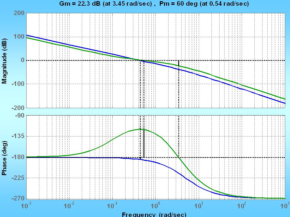
50. Before design After design

51. Closed-loop Bode plot by: Magnitude plot shifted up 3dB So, gc is BW margin(ncl*1.414,dcl);

53. Alternative use of lead Use Lead and Proportional together –To fix overshoot and ess –No speed requirement 1.Select K so that KG(s) meet ess req. 2.Find wgc and PM, also find PMd 3.Determine phi_max, and alpha 4.Place phi_max a little higher than wgc

54. Alternative lead design example Plant transfer function is given by: n=[50]; d=[1/50 1 0]; Desired design specifications are: –Step response overshoot <= 20% –Steady state tracking error for ramp input <= 1/200; –No speed requirements –No settling concern –No bandwidth requirement

55. n=[50]; d=[1/5 1 0]; figure(1); clf; margin(n,d); grid; hold on; Mp = 20/100; zeta = sqrt((log(Mp))^2/(pi^2+(log(Mp))^2)); PMd = zeta * 100 + 10; ess2ramp= 1/200; Kvd=1/ess2ramp; Kva = n(end)/d(end-1); Kzp = Kvd/Kva; figure(2); margin(Kzp*n,d); grid; [GM,PM,wpc,wgc]=margin(Kzp*n,d); w_gcd=wgc; phimax = (PMd-PM)*pi/180; alpha=(1+sin(phimax))/(1-sin(phimax)); z=w_gcd/alpha^.25; %sqrt(alpha); %phimax located higher p=w_gcd*alpha^.75; %sqrt(alpha); %than wgc ngc = conv(n, alpha*Kzp*[1 z]); dgc = conv(d, [1 p]); figure(3); margin(tf(ngc,dgc)); grid; [ncl,dcl]=feedback(ngc,dgc,1,1); figure(4); step(ncl,dcl); grid; figure(5); margin(ncl*1.414,dcl); grid;

62. Lead design tuning example C(s)G(s) Design specifications: rise time <=2 sec overshoot <16%

75. 4. Go back and take wgcd = 0.6*wn so that tr is not too small Desired tr < 2 sec We had tr = 1.14 in the previous 4 designs

76. n=[1]; d=[1 5 0 0]; G=tf(n,d); Mp_d = 16; %in percentage PMd = 70 - Mp_d + 4; %use Mp + PM =70 tr_d = 2; wnd = 1.8/tr_d; w_gcd = 0.6*wnd; Gwgc=evalfr(G, j*w_gcd); PM = pi+angle(Gwgc); phimax= PMd*pi/180-PM; alpha=(1+sin(phimax))/(1-sin(phimax)); zlead= w_gcd/sqrt(alpha); plead=w_gcd*sqrt(alpha); K=sqrt(alpha)/abs(Gwgc); ngc = conv(n, K*[1 zlead]); dgc = conv(d, [1 plead]); [ncl,dcl]=feedback(ngc,dgc,1,1); stepchar(ncl,dcl); grid figure(2); margin(G); hold on; margin(ngc,dgc); hold off; grid

79. Lead design C(s)G(s) Design specifications: Keep tr, td, but reduce overshoot to <16%

80. Lag design C(s)G(s) Desired design specifications are: –Step response overshoot <= 20% –Steady state tracking error for ramp input <= 1/200;

81. Alternative lead design example Plant transfer function is given by: n=[50]; d=[1/50 1 0]; Desired design specifications are: –Step response overshoot <= 20% –Steady state tracking error for ramp input <= 1/200; –No speed requirements –No settling concern –No bandwidth requirement