1. EA C461 - Artificial Intelligence
Neural Networks
EA C461 - Artificial Intelligence 1

2. Topics Connectionist Approach to Learning
Perceptron, Perceptron Learning 2

3. Neural Net example: ALVINN
Autonomous vehicle controlled by Artificial Neural Network
Drives up to 70mph on public highways
Note: most images are from the online slides for Tom Mitchell’s book “Machine Learning”

4. Neural Net example: ALVINN
Sharp left
Straight ahead
Sharp right
30 output units
4 hidden units
Learning means adjusting weight values
1 input pixel
Input is 30x32 pixels
= 960 values

5. Neural Net example: ALVINN
Output is array of 30 values
This corresponds to steering instructions
E.g. hard left, hard right
This shows one hidden node
Input is 30x32 array of pixel values
= 960 values
Note: no special visual processing
Size/colour corresponds to weight on link

6. Neural Networks
Mathematical representations of information processing in biological systems?
Efficient models for statistical pattern recognition
Multi Layer Perceptron
Model comprises multiple layers of logistic regression models (with continuous nonlinearities)
Compact models, comparing to SVM with similar generalization performances
Likelihood function is no longer convex!!!
Substantial resources requirement for training , often
Quicker processing of new data

7. Feed-forward Network Functions
Linear models for regression and classification
Neural networks use basis functions that follow similar form
Each basis function is itself a nonlinear function of a linear combination of the inputs,
The coefficients in the linear combination are adaptive parameters
Can be modeled as a series of functional transformations

8. Feed-forward Network Functions
First construct M linear combinations of the input variables x1 , , xD in the form
aj is called as activation, wj0 is bias, wji are weights
h(.) – non linear differentiable transformation
Generally sigmoid function : logic sigmoid, tanh

9. Feed-forward Network Functions
Proceed to do the same with the second layer
The choice of activation function at second layer (corresponds to output ) is determined by the nature of the data and the assumed distribution of target variables

10. Feed-forward Network Functions
Evaluating this equation can be interpreted as a forward propagation of information through the network
Bias can be absorbed into the input

11. Feed-forward Network

12. Activation functions Activation functions are linear for perceptrons
Activation functions are not linear for MLP
Composition of successive linear transformations is itself a linear transformation
We can always find an equivalent network without hidden units
If the number of hidden units is smaller than either the number of input or output units, then
the information is lost in the dimensionality reduction at the hidden units.
the transformations that the network can generate are not the most general possible linear transformations from inputs to outputs because
Little / no interest in MLP’s with linear activation for hidden layers

13. Output layer
For regression we use linear outputs and a sum-of-squares error, for (multiple independent)
For binary classifications we use logistic sigmoid outputs and a cross-entropy error function, and for multiclass classification we use softmax outputs with the corresponding multiclass cross-entropy error function
For classification problems involving two classes, we can use a single logistic sigmoid output, or a network with two outputs having a softmax output activation function

14. Universal Approximators
A two-layer network with linear outputs can uniformly approximate any continuous function on a compact input domain to arbitrary accuracy provided the network has a sufficiently large number of hidden units
Universal approximators

15. Parameter optimization
In the neural networks literature, it is usual to consider the minimization of an error function rather than the maximization of the (log) likelihood
Maximizing the likelihood function is equivalent to minimizing the sum-of-squares error function

16. Parameter optimization
The value of w found by minimizing E( w ) will be denoted wML because it corresponds to the maximum likelihood solution.
The nonlinearity of the network function y( xn, w ) causes the error E( w ) to be nonconvex
In practice local maxima of the likelihood may be found,

17. Parameter optimization

18. Parameter optimization
If we make a small step in weight space from w to w+δ w then the change in the error function is
δE ≈ δwT ∇E(w)
where
∇E(w) points in the direction of greatest rate of increase of the error function.
A step in the direction of −∇E(w) reduces the error

19. Parameter optimization
E(w) is a smooth continuous function of w
It’s value will be smaller where the gradient of the error function vanishes , i.e E(w) = 0 , stationary point
Stationary points can be minima, maxima & saddle points
Many points in weight space at which the gradient vanishes
For any point w that is a local minimum, there will be other points in weight space that are equivalent minima
In a two-layer network with M hidden units, each point in weight space is a member of a family of M!2M equivalent points (plus) multiple inequivalent stationary points and multiple inequivalent minima

20. Parameter optimization
Not always feasible to find the global minimum
Also, it will not be known whether the global minimum has been found
It may be necessary to compare several local minima in order to find a sufficiently good solution
Iterative numerical procedures
Choose some initial value w(0) for the weight vector
Navigate through weight space in a succession of steps of the form
w (τ +1) = w(τ) + ∆w(τ)
τ – Iteration Step
The value of ∇E(w) is evaluated at the new weight vector w(τ+1)

21. Gradient descent optimization
Update weight to make a small step in the direction of the negative gradient
Error function is defined with respect to a training set
Each step requires that the entire training set be processed to evaluate ∇E
Batch methods
It is necessary to run gradient-based algorithm multiple times
Each time using a different randomly chosen starting point
Comparing the resulting performance on an independent validation set

22. Gradient descent optimization
Error functions based on ML principle for a set of independent observations comprise a sum of terms, one for each data point
On-line gradient descent / sequential gradient descent / stochastic gradient descent, makes an update to the weight vector based on one data point at a time
Cycle through each point/ pick random points with replacement

23. Back propagation

24. Back propagation – misc slides

26. Regularization in Neural Networks
The generalization error is not a simple function of M due to the presence of local minima in the error function
Not always feasible to choose M by plotting

27. Regularization in Neural Networks
The number of input and outputs units in a neural network is determined by the dimensionality of the data set
The number M of hidden units is a free parameter that can be adjusted to give the best predictive performance

28. Regularization in Neural Networks
Choose a relatively large value for M and then control the complexity by the addition of a regularization term to the error function
The simplest regularizer is the quadratic
Weight decay regularizer
The effective model complexity is determined by the choice of the regularization coefficient λ

29. Early Stopping
Training can therefore be stopped at the point of smallest error with respect to the validation data set

30. Invariance
In the classification of objects in two-dimensional images, such as handwritten digits, a particular object should be assigned the same classification irrespective of its
position within the image (translation invariance)
its size (scale invariance)
If sufficiently large numbers of training patterns are available, then neural network can learn the invariance(at least approximately)

31. Invariance
Can we augment the training set using replicas of the training patterns, transformed according to the desired invariances

32. Invariance We can simply ignore the invariance in the neural network
Invariance is built into the pre-processing by extracting features that are invariant under the required transformations
Any subsequent regression or classification system that uses such features as inputs will necessarily also respect these invariances
Build the invariance properties into the structure of a neural network  Convolutional neural networks
Idea:
Extracting local features that depend only on small subregions
Merge these info in later stages of processing in order to detect higher-order features  ultimately as the image as a whole

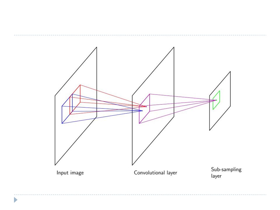
34. Convolutional neural networks
Build the invariance properties into the structure of a neural network  Convolutional neural networks
Idea:
Extracting local features that depend only on small subregions
Merge these info in later stages of processing in order to detect higher-order features  ultimately as the image as a whole

35. Radial Basis Function An approach to function approximation
Learned hypothesis takes the form
k  user provided constant (Number of Kernels)
xu is an intance from X.
Ku will decrease with d increases, and generally it is a Gaussian Kernel, centered at xu

36. Radial Basis Functions
This function can be used to describe a two- layer network
The width of each kernel σ2 can be separately specified
The network training procedure learns wi.

37. Radial Basis Functions
Choosing kernels
One fixed width kernel for each training point
Each kernel influences the only its neighborhood
Fits training data exactly
Choose smaller number of kernels in comparison with the number of training examples
Each kernel distributed uniformly across the space (or) guided by the EM Algorithm

38. Radial Basis Function Summarization on RBF
Provides a global approximation to the target function
Represented by a linear combination of many local kernel functions
To neglect the values out of defined region(region/width)
Can be trained more efficiently