2. Why did home prices boom and bust? In July 2006, home prices in the United States peaked at double their 1999 level. By early 2009, prices had crashed by 46 percent and were back at their 2002 levels. Why? What made home prices rise and then fall?

3. © 2011 Pearson Education Demand and Supply 4 When you have completed your study of this chapter, you will be able to 1 Distinguish between quantity demanded and demand, and explain what determines demand. 2 Distinguish between quantity supplied and supply, and explain what determines supply. 3 Explain how demand and supply determine price and quantity in a market, and explain the effects of changes in demand and supply. CHAPTER CHECKLIST

4. COMPETITIVE MARKETS A market is any arrangement that bring buyers and sellers together. A market might be a physical place or a group of buyers and sellers spread around the world who never meet.

5. COMPETITIVE MARKETS In this chapter, we study a competitive market that has so many buyers and so many sellers that no individual buyer or seller can influence the price.

6. 4.1 DEMAND Quantity demanded is t he amount of a good, service, or resource that people are willing and able to buy during a specified period at a specified price. The quantity demanded is an amount per unit of time. For example, the amount per day or per month.

7. 4.1 DEMAND Law of Demand Other things remaining the same, If the price of the good rises, the quantity demanded of that good decreases. If the price of the good falls, the quantity demanded of that good increases.

8. 4.1 DEMAND Demand Schedule and Demand Curve Demand is the relationship between the quantity demanded and the price of a good when all other influences on buying plans remain the same. Demand is a list of quantities at different prices and is illustrated by the demand curve.

9. 4.1 DEMAND Demand schedule is a list of the quantities demanded at each different price when all the other influences on buying plans remain the same. Demand curve is a graph of the relationship between the quantity demanded of a good and its price when all other influences on buying plans remain the same.

10. 4.1 DEMAND

12. Individual Demand and Market Demand Market demand is the sum of the demands of all the buyers in a market. The market demand curve is the horizontal sum of the demand curves of all buyers in the market.

13. 4.1 DEMAND

15. Changes in Demand Change in demand is a change in the quantity that people plan to buy when any influence other than the price of the good changes. A change in demand means that there is a new demand schedule and a new demand curve.

16. 4.1 DEMAND Figure 4.3 shows changes in demand. 1.When demand decreases, the demand curve shifts leftward from D 0 to D 1. 2.When demand increases, the demand curve shifts rightward from D 0 to D 2.

18. 4.1 DEMAND The main influences on buying plans that change demand are Prices of related goods Expected future prices Income Expected future income and credit Number of buyers Preferences

19. 4.1 DEMAND Prices of Related Goods A substitute is a good that can be consumed in place of another good. For example, apples and oranges are substitutes. The demand for a good increases, if the price of one of its substitutes rises. The demand for a good decreases, if the price of one of its substitutes falls.

20. 4.1 DEMAND A complement is a good that is consumed with another good. For example, ice cream and fudge sauce are complements. The demand for a good increases, if the price of one of its complements falls. The demand for a good decreases, if the price of one of its complements rises.

21. 4.1 DEMAND Expected Future Prices A rise in the expected future price of a good increases the current demand for that good. A fall in the expected future price of a good decreases current demand for that good. For example, if the price of a computer is expected to fall next month, the demand for computers today decreases.

22. 4.1 DEMAND Income A normal good is a good for which the demand increases if income increases and demand decreases if income decreases. An inferior good is a good for which the demand decreases if income increases and demand increases if income decreases.

23. 4.1 DEMAND Expected Future Income and Credit When income is expected to increase in the future, or when credit is easy to get and the cost of borrowing is low, the demand for some goods increases. When income is expected to decrease in the future, or when credit is hard to get and the cost of borrowing is high, the demand for some goods decreases. Changes in expected future income and the availability and cost of credit has the greatest effect on the demand for big ticket items such as homes and cars.

24. 4.1 DEMAND Number of Buyers The greater the number of buyers in a market, the larger is the demand for any good. Preferences When preferences change, the demand for one item increases and the demand for another item (or items) decreases. Preferences change when: People become better informed. New goods become available.

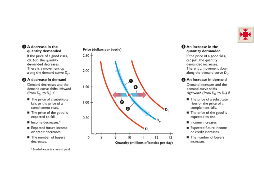
25. 4.1 DEMAND Change in Quantity Demanded Versus Change in Demand A change in the quantity demanded is a change in the quantity of a good that people plan to buy that results from a change in the price of the good. A change in demand is a change in the quantity that people plan to buy when any influence other than the price of the good changes.

26. 4.1 DEMAND Figure 4.4 illustrates and summarizes the distinction.

28. 4.2 SUPPLY Quantity supplied is the amount of a good, service, or resource that people are willing and able to sell during a specified period at a specified price. The Law of Supply Other things remaining the same, If the price of a good rises, the quantity supplied of that good increases. If the price of a good falls, the quantity supplied of that good decreases.

29. 4.2 SUPPLY Supply Schedule and Supply Curve Supply is the relationship between the quantity supplied of a good and the price of the good when all other influences on selling plans remain the same. Supply is a list of quantities at different prices and is illustrated by the supply curve.

30. 4.2 SUPPLY A supply schedule is a list of the quantities supplied at each different price when all other influences on selling plans remain the same. A supply curve is a graph of the relationship between the quantity supplied and the price of the good when all other influences on selling plans remain the same.

31. 4.2 SUPPLY

33. Individual Supply and Market Supply Market supply is the sum of the supplies of all sellers in a market. The market supply curve is the horizontal sum of the supply curves of all the sellers in the market.

34. 4.2 SUPPLY

36. Changes in Supply A change in supply is a change in the quantity that suppliers plan to sell when any influence on selling plans other than the price of the good changes. A change in supply means that there is a new supply schedule and a new supply curve.

37. 4.2 SUPPLY 2.When supply increases, the supply curve shifts rightward from S 0 to S 2. 1.When supply decreases, the supply curve shifts leftward from S 0 to S 1. Figure 4.7 shows changes in supply. 4.2 SUPPLY

39. The main influences on selling plans that change supply are Prices of related goods Prices of resources and other Inputs Expected future prices Number of sellers Productivity

40. 4.2 SUPPLY Prices of Related Goods A change in the price of one good can bring a change in the supply of another good. A substitute in production is a good that can be produced in place of another good. For example, a truck and an SUV are substitutes in production in an auto factory. The supply of a good increases if the price of one of its substitutes in production falls. The supply a good decreases if the price of one of its substitutes in production rises.

41. 4.2 SUPPLY A complement in production is a good that is produced along with another good. For example, cream is a complement in production of skim milk in a dairy. The supply of a good increases if the price of one of its complements in production rises. The supply a good decreases if the price of one of its complements in production falls.

42. 4.2 SUPPLY Prices of Resources and Other Inputs Resource and input prices influence the cost of production. And the more it costs to produce a good, the smaller is the quantity supplied of that good. Expected Future Prices Expectations about future prices influence supply. Expectations of future prices of resources also influence supply.

43. 4.2 SUPPLY Number of Sellers The greater the number of sellers in a market, the larger is supply. Productivity Productivity is output per unit of input. An increase in productivity lowers costs and increases supply. For example, an advance in technology increases supply. A decrease in productivity raises costs and decreases supply. For example, a severe hurricane decreases supply.

44. 4.2 SUPPLY Change in Quantity Supplied Versus Change in Supply A change in quantity supplied is a change in the quantity of a good that suppliers plan to sell that results from a change in the price of the good. A change in supply is a change in the quantity that suppliers plan to sell when any influence on selling plans other than the price of the good changes.

45. 4.2 SUPPLY Figure 4.8 illustrates and summarizes the distinction

47. 4.3 MARKET EQUILIBRIUM Market equilibrium occurs when the quantity demanded equals the quantity supplied. At market equilibrium, buyers and sellers plans are consistent. Equilibrium price is the price at which the quantity demanded equals the quantity supplied. Equilibrium quantity is the quantity bought and sold at the equilibrium price.

48. 4.3 MARKET EQUILIBRIUM Figure 4.9 shows the equilibrium price and equilibrium quantity. 1. Market equilibrium at theintersection of the demand curve and the supply curve. 2. The equilibrium price is $1 a bottle. 3. The equilibrium quantity is 10 million bottles a day.

50. 4.3 MARKET EQUILIBRIUM Price: A Markets Automatic Regulator Law of market forces When there is a shortage, the price rises. When there is a surplus, the price falls. Shortage or Excess Demand is the quantity demanded exceeds the quantity supplied. Surplus or Excess Supply is the quantity supplied exceeds the quantity demanded.

51. 4.3 MARKET EQUILIBRIUM Figure 4.10(a) market achieves equilibrium. At $1.50 a bottle: 1. Quantity is supplied 11 million bottles. 3. There is a surplus of 2 million bottles. 4. Price falls until the surplus is eliminated and the market is in equilibrium. 2. Quantity demanded is 9 million bottles.

53. 4.3 MARKET EQUILIBRIUM Figure 4.10(b) market achieves equilibrium. At 75 cents a bottle: 1. Quantity demanded is 11 million bottles. 3. There is a shortage of 2 million bottles. 4. Price rises until the shortage is eliminated and the market is in equilibrium. 2. Quantity supplied is 9 million bottles.

55. 4.3 MARKET EQUILIBRIUM Predicting Price Changes: Three Questions We can work out the effects of an event by answering: 1.Does the event change demand or supply? 2.Does the event increase or decrease demand or supplyshift the demand curve or the supply curve rightward or leftward? 3.What are the new equilibrium price and equilibrium quantity and how have they changed?

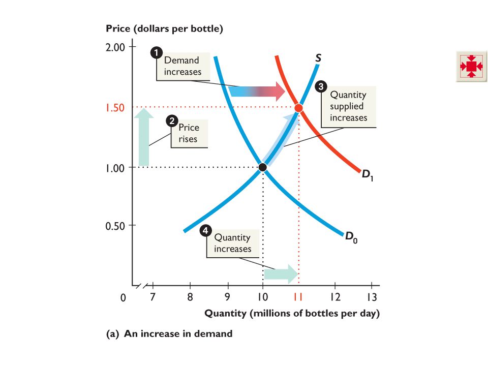
56. 4.3 MARKET EQUILIBRIUM Effects of Changes in Demand Event: A new study says that tap water is unsafe. In the market for bottled water: 1.With tap water unsafe, demand for bottled water changes. 2.The demand for bottled water increases, the demand curve shifts rightward. 3.What are the new equilibrium price and equilibrium quantity and how have they changed?

57. 4.3 MARKET EQUILIBRIUM Figure 4.11(a) illustrates the outcome. 1. An increase in demand shifts the demand curve rightward. 2. At $1.00 a bottle, there is a shortage, so the price rises. 3. The quantity supplied increases along the supply curve. 4. Equilibrium quantity increases.

59. 4.3 MARKET EQUILIBRIUM Event: A new zero-calorie sports drink is invented. In the market for bottled water: 1.The new drink is a substitute for bottled water, so the demand for bottled water changes 2.The demand for bottled water decreases, the demand curve shifts leftward. 3.What are the new equilibrium price and equilibrium quantity and how have they changed?

60. 4.3 MARKET EQUILIBRIUM Figure 4.11(b) shows the outcome. 1. A decrease in demand shifts the demand curve leftward. 2. At $1.00 a bottle, there is a surplus, so the price falls. 3. Quantity supplied decreases along the supply curve. 4. Equilibrium quantity decreases.

62. 4.3 MARKET EQUILIBRIUM When demand changes: The supply curve does not shift. But there is a change in the quantity supplied. Equilibrium price and equilibrium quantity change in the same direction as the change in demand.

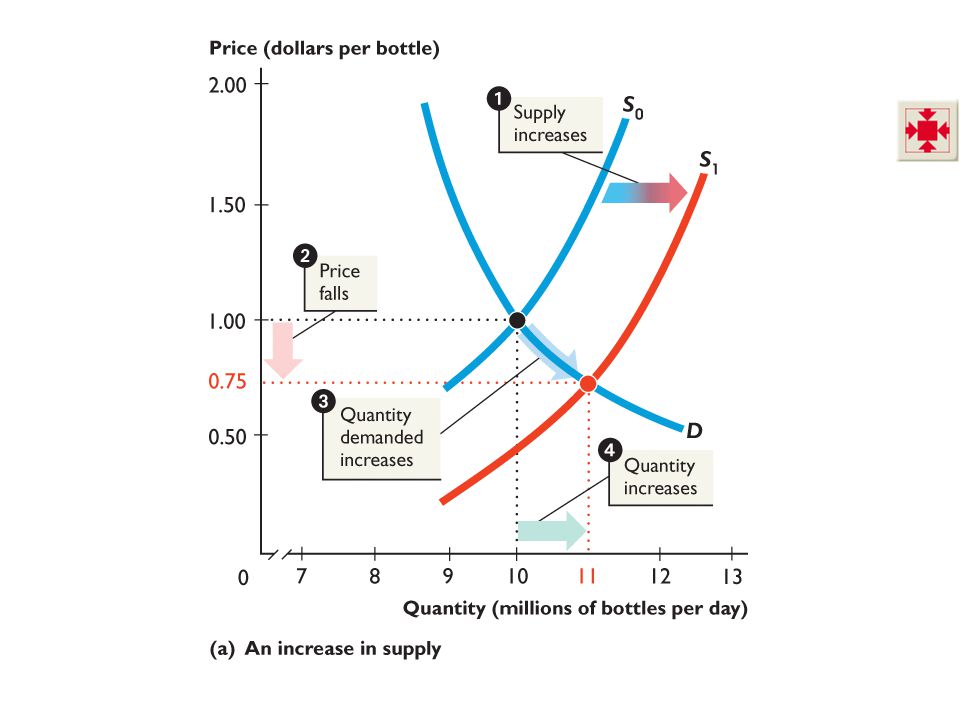
63. 4.3 MARKET EQUILIBRIUM Effects of Changes in Supply Event: Europeans water bottlers buy springs and open plants in the United States. In the market for bottled water: 1.With more suppliers of bottled water, supply changes. 2.The supply of bottled water increases, the supply curve shifts rightward. 3.What are the new equilibrium price and equilibrium quantity and how have they changed?

64. 4.3 MARKET EQUILIBRIUM Figure 4.12(a) shows the outcome. 1. An increase in supply shifts the supply curve rightward. 2. At $1.00 a bottle, there is a surplus, so the price falls. 3. Quantity demanded increases along the demand curve. 4. Equilibrium quantity increases.

66. 4.3 MARKET EQUILIBRIUM Event: Drought dries up some springs in the United States. In the market for bottled water: 1. Drought changes the supply of bottled water. 2. The supply of bottled water decreases, the supply curve shifts leftward. 3. What are the new equilibrium price and equilibrium quantity and how have they changed?

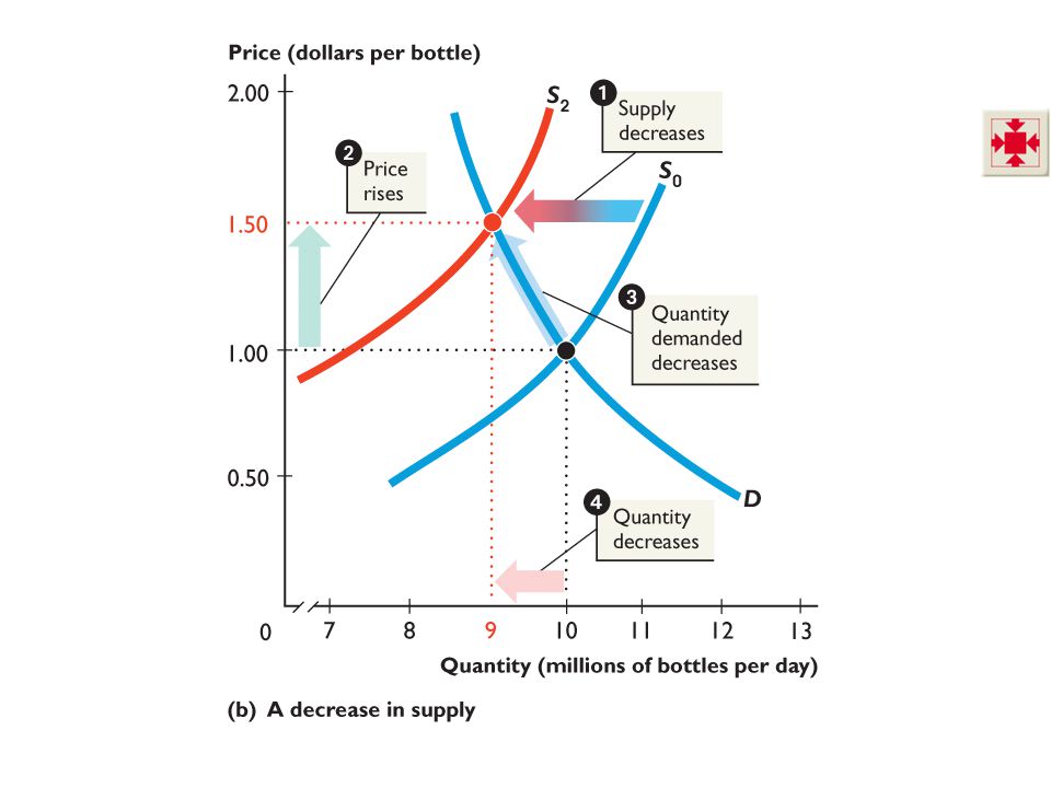
67. 4.3 MARKET EQUILIBRIUM Figure 4.12(b) shows the outcome. 1. A decrease in supply shifts the supply curve leftward. 2. At $1.00 a bottle, there is a shortage, so the price rises. 3. Quantity demanded decreases along the demand curve. 4. Equilibrium quantity decreases.

69. 4.3 MARKET EQUILIBRIUM When supply changes: The demand curve does not shift. But there is a change in the quantity demanded. Equilibrium price changes in the same direction as the change in supply. Equilibrium quantity changes in the opposite direction to the change in supply.

70. 4.3 MARKET EQUILIBRIUM Changes in Both Demand and Supply When two events occur at the same time, work out how each event influences the market: 1.Does each event change demand or supply? 2.Does either event increase or decrease demand or increase or decrease supply? 3.What are the new equilibrium price and equilibrium quantity and how have they changed?

71. 4.3 MARKET EQUILIBRIUM The figure shows the effects of an increase in both demand and supply. An increase in demand shifts the demand curve rightward; an increase in supply shifts the supply curve rightward. 1. Equilibrium quantity increases. 2. Equilibrium price might rise or fall.

73. 4.3 MARKET EQUILIBRIUM Increase in Both Demand and Supply Increases the equilibrium quantity. The change in the equilibrium price is ambiguous because the: Increase in demand raises the price. Increase in supply lowers the price.

74. 4.3 MARKET EQUILIBRIUM This figure shows the effects of a decrease in both demand and supply. A decrease in demand shifts the demand curve leftward; a decrease in supply shifts the supply curve leftward. 1. Equilibrium quantity decreases. 2. Equilibrium price might rise or fall.

76. 4.3 MARKET EQUILIBRIUM Decrease in Both Demand and Supply Decreases the equilibrium quantity. The change in the equilibrium price is ambiguous because the: Decrease in demand lowers the price Decrease in supply raises the price.

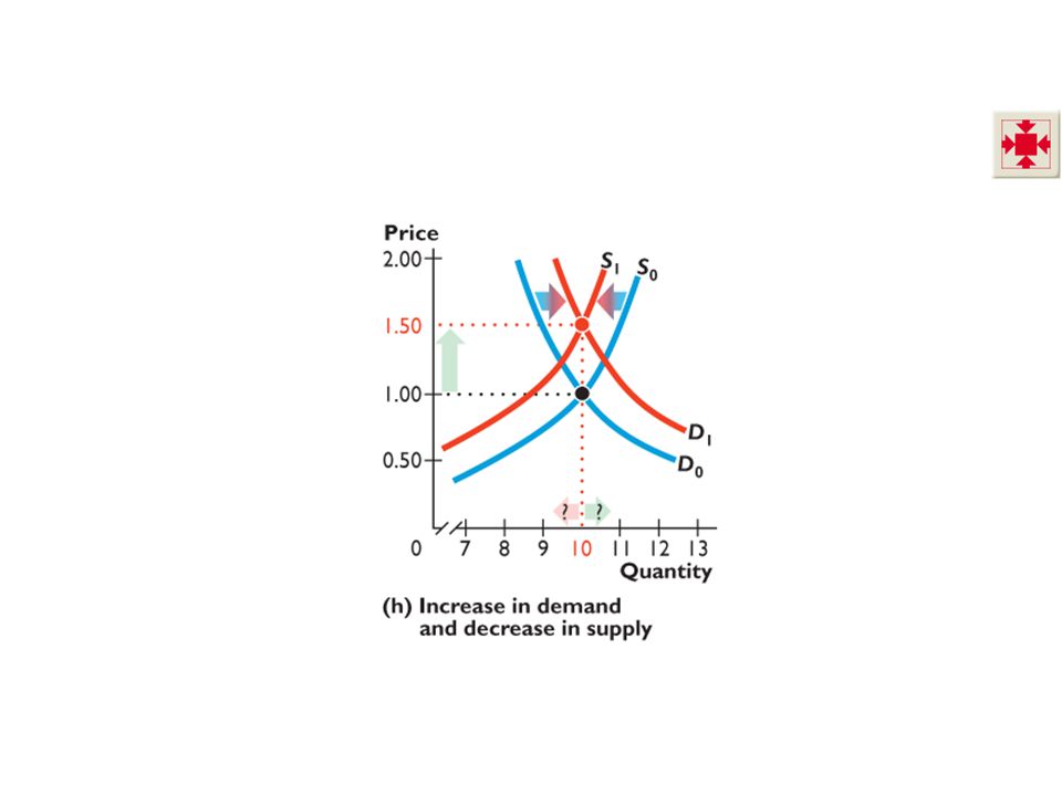
77. 4.3 MARKET EQUILIBRIUM The figure shows the effects of an increase in demand and a decrease in supply. An increase in demand shifts the demand curve rightward; a decrease in supply shifts the supply curve leftward. 1. Equilibrium price rises. 2. Equilibrium quantity might increase, decrease, or not change.

79. 4.3 MARKET EQUILIBRIUM Increase in Demand and Decrease in Supply Raises the equilibrium price. The change in the equilibrium quantity is ambiguous because the: Increase in demand increases the quantity. Decrease in supply decreases the quantity.

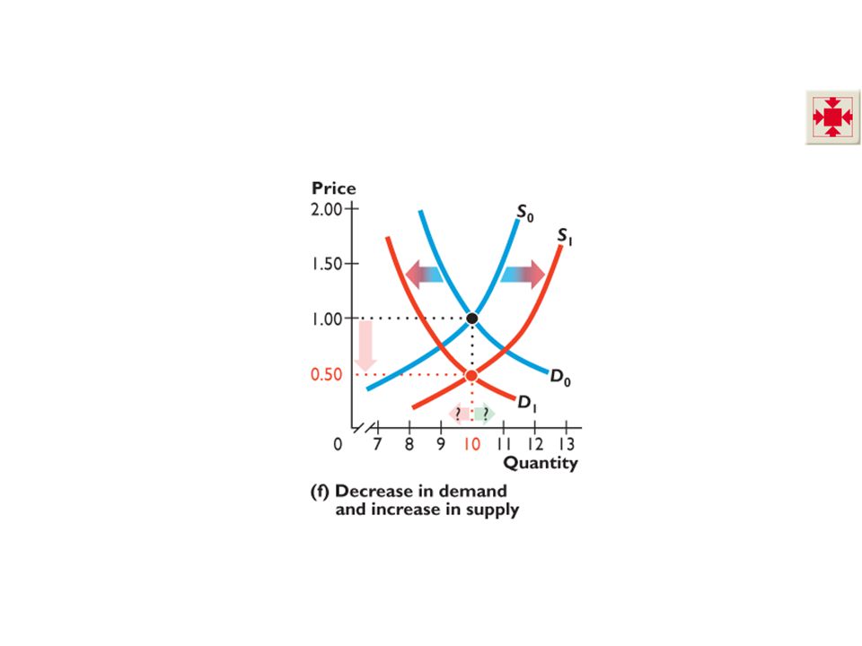
80. 4.3 MARKET EQUILIBRIUM This figure shows the effects of a decrease in demand and an increase in supply. A decrease in demand shifts the demand curve leftward; an increase in supply shifts the supply curve rightward. 1. Equilibrium price falls. 2. Equilibrium quantity might increase, decrease, or not change.

82. 4.3 MARKET EQUILIBRIUM Decrease in Demand and Increase in Supply Lowers the equilibrium price. The change in the equilibrium quantity is ambiguous because the: Decrease in demand decreases the quantity. Increase in supply increases the quantity.

83. In 1999, the price of an average home was $200,000, but home prices were rising by almost 10 percent a year. The pace of increase picked up and by 2004, home prices were rising by 15 percent a year. What caused this boom in home prices? Why Did Home Prices Boom and Bust? EYE on HOME PRICES

84. 1.Cheap and easy loans increased the demand for homes. 2.With house prices expected to rise further he supply of homes for sale decreased. 3. Home prices soared. In 2006, home prices started to fall. What caused home prices to fall? Why Did Home Prices Boom and Bust? EYE on HOME PRICES

85. 1.Cheap and easy loans dried up the demand for homes. 2.With house prices expected to fall the supply of homes for sale increased. 3. Home prices fell. By 2009, the average home price had fallen to 54 percent of the 2006 peak value. Why Did Home Prices Boom and Bust? EYE on HOME PRICES