1. Presented by: Bhavin Gandhi Jaime Tibaduiza Althea Lim Sean Findley

2. Does the Stock Market Overreact? ByWerner F. M. De Bondt; Richard Thaler

3. Does the stock market overreact? Most people overreact to unexpected events CRSP monthly return data is consistent with that This is a violation of Bayes rule Definition of Bayes rule Example of Bayes rule

4. Individual psychology and market behavior What is an overreaction? Kahneman and Tversky: Representativeness heuristic Observation by J. M. Keynes Theory of investment value by Williams

5. Price to earnings (P/E) ratio anomaly Dividends do not vary significantly to justify stock price movement Correlation between stock prices and following years earnings Investors attach misappropriate importance to short- run Alternative explanation given by Basu: price-ratio hypothesis

6. The overreaction hypothesis: Empirical Tests Test of semi-strong form of market starts at t = 0 Formation of portfolio on basis of some event affecting all portfolios (e.g.: earnings) Measurement of residual portfolio return at t>0 = 0 Results can be affected by CAPM, poor estimation of alpha and beta, weak-form inefficiency

7. Test assessed in this study Systematic nonzero residual return after portfolio formation (t>0) Association with systematic residual returns in pre- formation (t<0) Focus on stocks with extreme movements Create two different portfolio on past returns Extreme capital gains – Winner (W) Extreme capital loss – Looser (L)

8. The Overreaction Hypothesis: Empirical Results The results of the tests developed in Section I are consistent with the overreaction hypothesis. Over the last half-century, loser portfolios of 35 stocks outperform the market by, on average, 19.6%, 36 months after portfolio formation.

9. The Overreaction Hypothesis: Empirical Results (Cont) Winner portfolios, on the other hand, earn about 5.0% less than the market. The difference in cumulative average The residual between the extreme portfolios, [ACAR L,36 - ACAR W,36 ] equals 24.6% (t-statistic: 2.20).

10. 19.6 -5.0

11. Main Findings The overreaction effect is asymmetric; it is much larger for losers than for winners. Most of the excess returns are realized in January. In months t = 1,t = 13, and t = 25, the loser portfolio earns excess returns of, respectively, 8.1% (t-statistic: 3.21), 5.6% (3.07), and 4.0% (2.76)

12. Main Findings (Cont) The overreaction phenomenon mostly occurs during the second and third year of the test period. Twelve months into the test period, the difference in performance between the extreme portfolios is only 5.4% (t-statistic: 0.77).

13. 8.1% (t-statistic: 3.21) 5.6% (t-statistic: 3.07) 4.0% (t-statistic: 2.76)

15. 16 Three-year formation period 24 Two-year formation period 49 One-year formation period

16. Main Findings (Cont) Table I and Figure 2 further indicate that the overreaction phenomenon is qualitatively different from the January effect and, more generally, from seasonality in stock prices.

17. Main Findings (Cont) Throughout the test period, the difference in ACAR for the experiment with a three-year formation period exceeds the same statistic for the experiments based on two- and one-year formation periods. But all three experiments are clearly affected by the same underlying seasonal pattern.

18. Main Findings (Cont) For the three-year experiment illustrated in Figure 1, the relevant numbers are respectively, 1.369 and 1.026 (t-statistic on the difference: 3.09), thus: the loser portfolios not only outperform the winner portfolios; if the CAPM is correct, they are also significantly less risky. From a different viewpoint, therefore, the results in Table I are likely to underestimate both the true magnitude and statistical significance of the overreaction effect.

19. Main Findings (Cont) The problem is particularly severe with respect to the winner portfolio. Rather than 1.369, the residual return calculations assume the CAPM-beta of that portfolio to equal 1.00 only. This systematic bias may be responsible for the earlier observed asymmetry in the return behavior of the extreme portfolios.

20. Main Findings (Cont) To reiterate, the previous findings are broadly consistent with the predictions of the overreaction hypothesis. However, several aspects of the results remain without adequate explanation. Most importantly, the extraordinarily large positive excess returns earned by the loser portfolio in January.

21. Main Findings (Cont) One method that allows us to further accentuate the strength of the January effect is to increase the number of replications. Figure 3 shows the ACAR's for an experiment with a five-year-long test period. Every December between 1932 and 1977, winner and loser portfolios are formed on the basis of residual return behavior over the previous five years. Clearly, the successive 46 yearly selections are not independent. Therefore, no statistical tests are performed.

23. Main Findings (Cont) The results in Figure 3 have some of the properties of a "trading rule." They represent the average (cumulative) excess return (before transaction costs) that an investor, aware of the overreaction phenomenon, could expect to earn following any December in which he chose to try the strategy. The effect of multiplying the number of replications is to remove part of the random noise.

24. Main Findings (Cont) The outstanding feature of Figure 3 is, once again, the January returns on the loser portfolio. The effect is observed as late as five Januaries after portfolio formation. Careful examination of Figure 3 also reveals a tendency, on the part of the loser portfolio, to decline in value (relative to the market) between October and December.

25. Main Findings (Cont) This observation is in agreement with the naive version of the tax-loss selling hypothesis as explained by Schwert. The winner portfolio, on the other hand, gains value at the end of the year and loses some in January

26. Conclusion Most people "overreact" to unexpected and dramatic news events. The question then arises whether such behavior matters at the market level Consistent with the predictions of the overreaction hypothesis, portfolios of prior "losers" are found to outperform prior "winners. Several aspects of the results remain without adequate explanation; most importantly, the large positive excess returns earned by the loser portfolio every January.

27. Returns to Buying Winners and Selling Losers: Implications for Stock Market Efficiency By Narasimhan Jegadeesh and Sheridan Titman

28. Contrarian Strategy Buying past losers Selling past winners Relative Strength Strategy Buying past winners Selling past losers

29. Section I - Trading Strategies Investigates the efficiency of the stock market by examining the profitability of a number of these strategies. Strategies: 1 st set of strategy (16 strategies) – include stocks based on their past 1, 2, 3, & 4 quarters and have holding periods that vary from 1 – 4 quarters. 2 nd set of strategy (16 strategies) – same as 1 st but this one skips a week between the portfolio formation period and the holding period.

30. Strategies include portfolios with overlapping holding periods. Select stocks on the basis of returns over the past J months and holds them for K months (J-month/K-month strategy). 10 decile portfolios, equally weigh Ascending order of the securities returns over the past J months. Top decile portfolio – losers Bottom decile portfolio – winners In each month t, buy winner portfolio and sell lower portfolio, holding for K months. Closes out the position initiated in month t – K.

31. Section II - The Returns of Relative Strength Portfolios Zero-cost portfolios are positive. Most successful zero-cost strategy selects stocks based on their returns over the previous 12 months, held for 3 months. The 6-month formation period produce returns of about 1% per month regardless of the holding period. On average Relative Strength Strategies are profitable. Table 1

32. Section III - Sources of Relative Strength Profits To decompose the excess returns documented in the last section & identify the important sources of relative strength profits. 1 st model Allows for factor-mimicking portfolio returns to be serially correlated but requires individual stocks to react instantaneously to factor realizations. Used to decompose Relative Strength profits into 2 components relating to systematic risk, which would exist in an efficient market, and a 3 rd component relating to firm-specific returns, which would contribute to Relative Strength Profits only if the market were inefficient.

33. 2 nd model Relaxes the assumption that stock react instantaneously to the common factor. Enables us to evaluate the possibility that the relative strength profits arise because of the a lead-lag relationship in stock prices similar to that proposed by Lo & Mackinlay (1990) as a partial explanation for short horizons contrarian profits.

34. In table 1, the performance of the relative strength strategies implies that stocks that generate higher than average returns in one period also generate higher than average returns in the period that follows. This equation equals the expected profits from the zero-cost contrarian trading strategy tested by Lehmann (1990) and Lo and Mackinley (1990) called the weighted relative strength strategy (WRSS), which is closely related to relative strength strategy.

35. 3 Potential Sources Cross-sectional dispersion in expected returns Securities that experience relatively high returns in 1 period can be expected to have high than avg. returns in the following period. Potential in Time – Factor If the factor portfolio returns exhibit positive serial correlation, the relative strength strategy will tend to pick stocks with high betas when the conditional expectation of the factor portfolio returns is high. Average serial covariance of the idiosyncratic components of security returns

36. Relative Strength Profits = Market Inefficiency? Need to identify the source of the profit If due to reason 1 or 2, there may be attributed to compensation for bearing systematic risk and need not be an indication of market inefficiency. If due to reason 3, results would suggest to market inefficiency.

37. The Average Size and Beta of Relative Strength Portfolios Does this strategy systematically pick high-risk stocks?

38. Lead-lag Effects and Relative Strength Profits - They got a negative relation between the relative strength profits and lagged square market. - Lead-lag effects is not an important source of relative strength profits.

39. The Serial Covariance of 6-Month Returns Is the answer to this equation positive? The serial covariance of 6-month returns of the equally weighted index is – 0.0028, which means that the serial covariance of factor portfolio returns is unlikely the source of relative strength profits.

40. Profits of the Relative Strength Strategy is related to market underreaction to the firm-specific information.

41. Section IV – Profitability of Relative Strength Strategies Within Size- and Beta-Based Subsamples Three-size based subsamples – small, medium, large Three beta-based subsamples – low-beta, medium- beta, and high-beta stocks Does the size and beta of the portfolio make a difference? If yes, then expected returns will be less within this subsamples then in full sample.

43. The abnormal returns are of approximately the same magnitude. Somewhat related to firm size and beta. For the zero-cost, winners minus the losers portfolio, subsample with largest firms generate lower abnormal returns (compared to the other 2) and the returns segmented by beta are monotonically increasing in beta. Evidence suggests that the profits are not primarily due to the serial correlation in the firm-specific component of returns. Profitability of this strategy is not confined to any particular subsample of stocks.

45. The abnormal performance of the zero-cost portfolio is due to the buy side of the transaction rather then the sell side. When the value-weighted index is used as the benchmark: Past winners >> significant positive abnormal returns. Past losers >> not statistically significant abnormal returns.

46. Section V: Sub Period Analysis Seasonal patterns in relative strength portfolio returns Conjecture is that relative strength patterns will not be successful in the month of January Magnitude of the negative January performance of the relative strength strategy to be inversely related to firm size The negative average relative strength return in January is not statistically significant for the subsample of large firms.

47. Section V: Sub Period Analysis For Table IV: The relative strength portfolios are formed based on 6-month lagged returns and held for 6 months. The stocks are ranked in ascending order on the basis of 6-month lagged returns The equally weighted portfolio of stocks in the lowest past return decile is the sell portfolio The equally weighted portfolio of stocks in the highest past return decile is the buy portfolio.

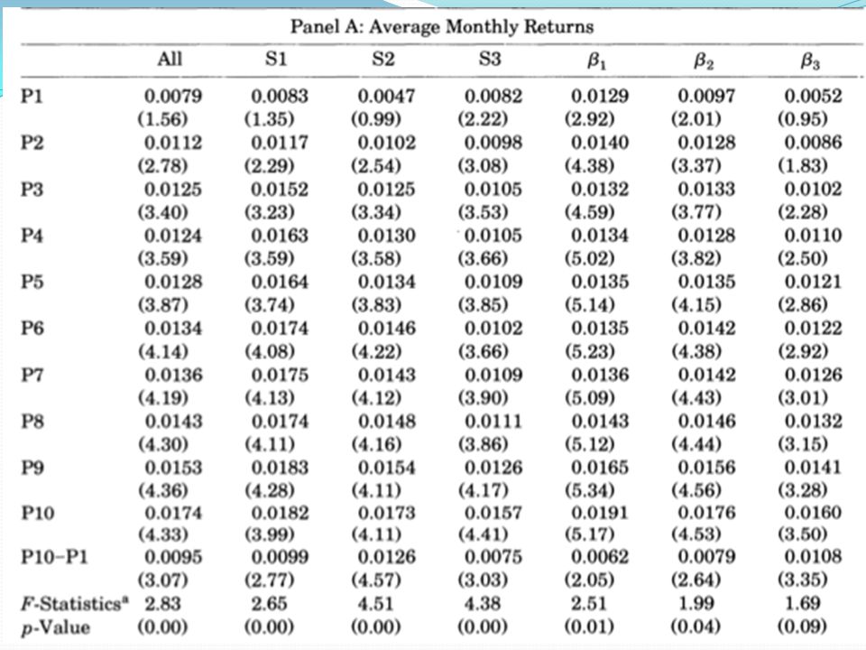
48. Section V: Sub Period Analysis Table IV reports the average monthly returns of the zero-cost, buy minus sell, portfolio in each calendar month. The average returns of the zero-cost portfolios formed using size-based subsamples of securities are also reported. The subsample S1 contains the smallest firms, S2 contains the medium-sized firms, and S3 contains the largest firms. The sample period is January 1965 to December 1989

49. Table IV: Returns on Size-Based Relative Strength Portfolios (P10-PI) by Calendar Months

50. Section V: Sub Period Analysis The negative average relative strength return in January is not statistically significant for the subsample of large firms. The findings in Table IV suggest that there is also a seasonal pattern outside January. For example, the returns are fairly low in August and are particularly high in April, November, and December. The F-statistics reported in this table indicate that these monthly differences outside January are statistically significant for the whole sample as well as for the sample of medium-size firms.

51. Section V: Sub Period Analysis One of the interesting findings documented in Table IV is that the relative strength strategy produces positive returns in 96% (24 out of 25) of the Aprils. The large (3.33%) and consistently positive April returns may be related to the fact that corporations must transfer money to their pension funds prior to April 15 if the funds are to qualify for a tax deduction in the previous year. If these pension fund assets are primarily invested by portfolio managers who follow relative strength rules, then the winners portfolio may benefit from additional price pressure in this month. Similarly, the larger than average returns in November and December may in part be due to price pressure arising from portfolio managers selling their losers in these months for tax or window dressing reasons.

52. Section V: Sub Period Analysis Table V: The relative strength portfolios are formed based on 6-month lagged returns and held for 6months. The stocks are ranked in ascending order on the basis of 6-month lagged returns and the equally weighted portfolio of stocks in the lowest past return decile is the sell portfolio The equally weighted portfolio of stocks in the highest past return decile is the buy portfolio.

53. Section V: Sub Period Analysis Table V reports the proportion of months when the average return of the zero-cost, buy minus sell, portfolio is positive. This proportion for the zero-cost portfolio formed within each size-based subsample of securities is also reported. The subsample S1 contains the smallest firms, S2 contains the medium-sized firms, and S3 contains the largest firms. The sample period is January 1965 to December 1989.

54. Table V: Proportion of Positive Returns of Relative Strength Portfolios by Calendar Months The relative strength strategy realizes positive returns in 67% of the months, and 71% of the months when January is excluded The relative strength strategy loses about 7% on average in each January but achieves positive abnormal returns in each of the other months The average return in non-January months is 1.66% per month. Magnitude of the negative January performance of the relative strength strategy to be inversely related to firm size (other research supports this).

55. Table VI: Proportion of Positive Returns of Relative Strength Portfolios by Calendar Months Average returns that are positive in all but one time period (1975 to 1979) Negative January returns during this period January are from small firms Positive profits in each of the five year periods for medium and large firms especially when January is excluded

56. Track the average portfolio returns in each of the 36 months following the portfolio formation date Test riskiness of the strategy and about whether the profits are due to overreaction or underreaction Are higher than average unconditional returns either because of their risk or for other reasons such as differential tax exposures? Significant negative returns of the zero-cost portfolio in the months following the holding period would suggest that the price changes during the holding period are at least partially temporary. One Possibility of the inverted U-Shape in next table is that the risk of strategy changes over event time Section VI: Performance of Relative Strength Portfolios in Event Time

57. Table VII: Performance of Relative Strength Portfolios in Event Time With the exception of month 1, the average return in each month is positive in the first year. The average return is negative in each month in year 2 as well as in the first half of year 3 and virtually zero thereafter. The cumulative returns reach a maximum of 9.5% at the end of 12 months but decline to about 4% by the end of month 36.

58. The negative returns beyond month 12 indicate that the relative strength strategy does not tend to pick stocks that have high unconditional expected returns. The observed pattern of initially positive and then negative returns of the zero-cost portfolio also suggests that the observed price changes in the first 12 months after the formation period may not be permanent. Unfortunately, estimates of expected returns over 2-year periods are not very precise. As a result, the negative returns for the zero-cost portfolio in years 2 and 3 are not statistically significant (t-statistic of - 1.27). Similarly, since the abnormal return over the entire 36-month period is not statistically different from zero, we cannot rule out the possibility that the positive returns over the first 12 months is entirely temporary. Section VI: Performance of Relative Strength Portfolios in Event Time

59. Section VII: Back-Testing the Strategy Replicate the test in Table VII, which tracks the performance of the 6-month relative strength portfolio in event time for both the 1927 to 1940 time period and the 1941 to 1964 time period Market was extremely volatile and experienced a significant degree of mean reversion in the 1927 to 1940 period In contrast, the market's volatility in the 1941 to 1964 period was similar to the volatility in the 1965 to 1989 period and the market index did not exhibit mean reversion in the post-1940 period.

60. Table VIII Panel A: Back-Testing the Strategy: Performance of Relative Strength Portfolios Prior to 1965 The returns in this time period are significantly lower than the returns in the 1965 to 1989 period, but the patterns of returns across event months is somewhat similar. Due to greater volatility during period; losers were close to bankruptcy, had high betas;

61. Table VIII Panel B: Back-Testing the Strategy: Performance of Relative Strength Portfolios Prior to 1965

62. Section VII: Back-Testing the Strategy The relative strength strategy returns over this time period are very similar to the returns in the more recent time period reported earlier. As in the 1965 to 1989 time period, the average return is slightly negative in month 1, significantly positive in month 2 through month 8, and negative in month 12 and beyond. In contrast to the findings for the 1965 to 1989 period, the positive cumulative return over the first 12 months dissipates almost entirely by month 24.

63. Section VIII: Stock Returns Around Earnings Announcement Dates This section examines the returns of past winners and losers around their quarterly earnings announcement dates. By analyzing stock returns within a short window around the dissemination of important firm-specific information we have a sharp test that directly assesses the potential biases in market expectations. For example, if stock price systems statistically underreact: In this case, the stock returns for past winners, which presumably had favorable information revealed in the past, should realize positive returns around the time when their earnings are actually announced. Similarly, past losers should realize negative returns around the time their earnings are announced

64. Section VIII: Stock Returns Around Earnings Announcement Dates The stocks are ranked in ascending order on the basis of 6- month lagged returns. The stocks in the lowest past return decile are called the losers group and the stocks in the highest past return decile is called the winners group. The differences between the 3-day returns (returns on days (-2 to 0) around quarterly earnings announcements for stocks in the winners group and the losers group are reported in table IX (rp - ri). t is the month after the ranking date. The sample period is January 1980 to December 1989.

65. Table IX: Quarterly Earnings Announcement Date Returns

66. Section VIII: Stock Returns Around Earnings Announcement Dates The pattern of announcement date returns presented in this table is consistent with the pattern of the zero-cost portfolio returns reported in Table VII. For the first 6 months the announcement date returns of the past winners exceed the announcement date returns of the past losers by over 0.7% on average, and is statistically significant in each of these 6 months. Since there are on average 2 quarterly earnings announcements per firm within a 6-month period, the returns around the earnings announcements represents about 25% of the zero-cost portfolio returns over this holding period.

67. Section VIII: Stock Returns Around Earnings Announcement Dates The negative announcement period returns in later months are consistent with the negative relative strength portfolio returns beyond month 12 documented earlier (see Table VII). From months 8 through 20 the differences in announcement date returns are negative and are generally statistically significant. The announcement period returns are especially significant in months 11 through 18 where they average about -0.7%. In the later months the differences between the announcement period returns of the winners and losers are generally negative but are close to zero.

68. Section VIII: Stock Returns Around Earnings Announcement Dates Bernard and Thomas find that average returns around quarterly earnings announcement dates are significantly positive following a favorable earnings surprise in the previous quarter. This is consistent with the positive announcement returns we see in the first 7 months in Table IX. Bernard and Thomas also find that the average return around earnings announcement dates is significantly negative 4 quarters after a positive earnings surprise. The significant negative returns around earnings announcement dates in months 11 through 18 in Table IX are consistent with this finding.

69. Conclusions Trading strategies that buy past winners and sell past losers realize significant abnormal returns over the 1965 to 1989 period. Not due to systematic risk. For example, the strategy we examine in most detail, which selects stocks based on their past 6-month returns and holds them for 6 months, realizes a compounded excess return of 12.01% per year on average. Specifically, stocks in the winners portfolio realize significantly higher returns than the stocks in the losers portfolio around the quarterly earnings announcements that are made in the first few months following the formation date. However, the announcement date returns in the 8 to 20 months following the formation date are significantly higher for the stocks in the losers portfolio than for the stocks in the winners portfolio. The evidence of initial positive and later negative relative strength returns suggests that common interpretations of return reversals as evidence of overreaction and return persistence (i.e., past winners achieving positive returns in the future) as evidence of underreaction are probably overly simplistic. A more sophisticated model of investor behavior is needed to explain the observed pattern of returns.