0. Economic Growth I: Capital Accumulation and Population Growth

1. What I want you to learn:
the closed economy Solow model
how a country’s standard of living depends on its saving and population growth rates
how to use the “Golden Rule” to find the optimal saving rate and capital stock 1

2. Why growth matters Data on infant mortality rates:
20% in the poorest 1/5 of all countries
0.4% in the richest 1/5
In Pakistan, 85% of people live on less than $2/day.
One-fourth of the poorest countries have had famines during the past 3 decades.
Poverty is associated with oppression of women and minorities.
Economic growth raises living standards and reduces poverty….

3. Income and poverty in the world selected countries, 2000

4. links to prepared graphs @ Gapminder.org
notes: circle size is proportional to population size, color of circle indicates continent
Income per capita and
Life expectancy
Infant mortality
Malaria deaths per 100,000
Adult literacy
Cell phone users per 100,000

5. Why growth matters
Anything that effects the long-run rate of economic growth – even by a tiny amount – will have huge effects on living standards in the long run.
percentage increase in standard of living after…
annual growth rate of income per capita
…25 years
…50 years
…100 years
2.0%
64.0%
169.2%
624.5%
2.5%
85.4%
243.7%
1,081.4%

6. Why growth matters
If the annual growth rate of U.S. real GDP per capita had been just one-tenth of one percent higher during the 1990s, the U.S. would have generated an additional $496 billion of income during that decade.

7. The lessons of growth theory
…can make a positive difference in the lives of hundreds of millions of people.
These lessons help us
understand why poor countries are poor
design policies that can help them grow
learn how our own growth rate is affected by shocks and our government’s policies

8. The Solow model
due to Robert Solow, won Nobel Prize for contributions to the study of economic growth
a major paradigm:
widely used in policy making
benchmark against which most recent growth theories are compared
looks at the determinants of economic growth and the standard of living in the long run

9. How Solow model is different from Chapter 3’s model
K is no longer fixed: investment causes it to grow, depreciation causes it to shrink
L is no longer fixed: population growth causes it to grow
the consumption function is simpler
no G or T (only to simplify presentation; we can still do fiscal policy experiments)
cosmetic differences

10. The production function
In aggregate terms: Y = F (K, L)
Define: y = Y/L = output per worker
k = K/L = capital per worker
Assume constant returns to scale: zY = F (zK, zL ) for any z > 0
Pick z = 1/L. Then
Y/L = F (K/L, 1)
y = F (k, 1)
y = f(k) where f(k) = F(k, 1)

11. The production function
Output per worker, y
Capital per worker, k
f(k) 1
MPK = f(k +1) – f(k)
Note: this production function exhibits diminishing MPK.

12. The national income identity
Y = C + I (remember, no G )
In “per worker” terms: y = c + i where c = C/L and i = I /L

13. The consumption function
s = the saving rate, the fraction of income that is saved
(s is an exogenous parameter)
Note: s is the only lowercase variable that is not equal to its uppercase version divided by L
Consumption function: c = (1–s)y (per worker)

14. Saving and investment saving (per worker) = y – c = y – (1–s)y = sy
National income identity is y = c + i
Rearrange to get: i = y – c = sy (investment = saving, like in chap. 3!)
Using the results above, i = sy = sf(k)

15. Output, consumption, and investment
Output per worker, y
Capital per worker, k
f(k) y1 k1 c1
sf(k) i1

16. Depreciation  = the rate of depreciation
= the fraction of the capital stock that wears out each period
Depreciation per worker, k
Capital per worker, k k  1

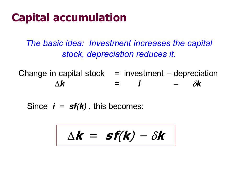
17. k = s f(k) – k Capital accumulation
The basic idea: Investment increases the capital stock, depreciation reduces it.
Change in capital stock = investment – depreciation
k = i – k
Since i = sf(k) , this becomes:
k = s f(k) – k

19. The equation of motion for k
k = s f(k) – k
The Solow model’s central equation
Determines behavior of capital over time…
…which, in turn, determines behavior of all of the other endogenous variables because they all depend on k. E.g.,
income per person: y = f(k)
consumption per person: c = (1–s) f(k)

20. k = s f(k) – k The steady state
If investment is just enough to cover depreciation [sf(k) = k ],
then capital per worker will remain constant: k = 0.
This occurs at one value of k, denoted k*, called the steady state capital stock.

21. Investment and depreciation
The steady state
Investment and depreciation
Capital per worker, k k
sf(k) k*

22. Moving toward the steady state
k = sf(k)  k
Investment and depreciation
Capital per worker, k k
sf(k) k*
investment k1 k
depreciation

23. Moving toward the steady state
k = sf(k)  k
Investment and depreciation
Capital per worker, k k
sf(k) k* k1 k k2

24. Moving toward the steady state
k = sf(k)  k
Investment and depreciation
Capital per worker, k k
sf(k) k*
investment k
depreciation k2

25. Moving toward the steady state
k = sf(k)  k
Investment and depreciation
Capital per worker, k k
sf(k) k* k2 k

26. Moving toward the steady state
k = sf(k)  k
Investment and depreciation
Capital per worker, k k
sf(k) k* k k2 k3

27. Moving toward the steady state
k = sf(k)  k
Investment and depreciation
Capital per worker, k k
Summary: As long as k < k*, investment will exceed depreciation, and k will continue to grow toward k*.
sf(k) k* k3

28. A numerical example Production function (aggregate):
To derive the per-worker production function, divide through by L:
Then substitute y = Y/L and k = K/L to get

29. A numerical example, cont.
Assume:
s = 0.3
 = 0.1
initial value of k = 4.0
As each assumption appears on the screen, explain it’s interpretation.
I.e.,
“The economy saves three-tenths of income,”
“every year, 10% of the capital stock wears out,” and
“suppose the economy starts out with four units of capital for every worker.”

30. Approaching the steady state: A numerical example
Year k y c i δk Δk … ∞
Before revealing the numbers in the first row, ask your students to determine them and write them in their notes. Give them a moment, then reveal the first row and make sure everyone understands where each number comes from.
Then, ask them to determine the numbers for the second row and write them in their notes.
After the second round of this, it’s probably fine to just show them the rest of the table.

31. NOW YOU TRY: Solve for the Steady State
Continue to assume s = 0.3,  = 0.1, and y = k 1/2
Use the equation of motion k = s f(k)  k to solve for the steady-state values of k, y, and c.

32. ANSWERS: Solve for the Steady State

33. An increase in the saving rate
An increase in the saving rate raises investment…
…causing k to grow toward a new steady state:
Investment and depreciation k δk
s2 f(k)
s1 f(k)

34. Prediction: Higher s  higher k*.
And since y = f(k) , higher k*  higher y* .
Thus, the Solow model predicts that countries with higher rates of saving and investment will have higher levels of capital and income per worker in the long run.

35. International evidence on investment rates and income per person
Income per person in (log scale)
Investment as percentage of output (average )

36. The Golden Rule: Introduction
Different values of s lead to different steady states. How do we know which is the “best” steady state?
The “best” steady state has the highest possible consumption per person: c* = (1–s) f(k*).
An increase in s
leads to higher k* and y*, which raises c*
reduces consumption’s share of income (1–s), which lowers c*.
So, how do we find the s and k* that maximize c*?

37. The Golden Rule capital stock
the Golden Rule level of capital, the steady state value of k that maximizes consumption.
To find it, first express c* in terms of k*:
c* = y*  i*
= f (k*)  i*
= f (k*)  k*
In the steady state: i* = k* because k = 0.

38. The Golden Rule capital stock
steady state output and depreciation
steady-state capital per worker, k*
 k*
Then, graph f(k*) and k*, look for the point where the gap between them is biggest.
f(k*)

39. The Golden Rule capital stock
c* = f(k*)  k* is biggest where the slope of the production function equals the slope of the depreciation line:
 k*
f(k*)
MPK = 
steady-state capital per worker, k*

40. The transition to the Golden Rule steady state
The economy does NOT have a tendency to move toward the Golden Rule steady state.
Achieving the Golden Rule requires that policymakers adjust s.
This adjustment leads to a new steady state with higher consumption.
But what happens to consumption during the transition to the Golden Rule?
Remember: policymakers can affect the national saving rate:
- changing G or T affects national saving
- holding T constant overall, but changing the structure of the tax system to provide more incentives for private saving (e.g., a revenue-neutral shift from the income tax to a consumption tax)

41. Starting with too much capital
then increasing c* requires a fall in s.
In the transition to the Golden Rule, consumption is higher at all points in time.
time y c i
t0 is the time period in which the saving rate is reduced. It would be helpful if you explained the behavior of each variable before t0, at t0 , and in the transition period (after t0 ).
Before t0: in a steady state, where k, y, c, and i are all constant.
At t0: The change in the saving rate doesn’t immediately change k, so y doesn’t change immediately. But the fall in s causes a fall in investment [because saving equals investment] and a rise in consumption [because c = (1-s)y, s has fallen but y has not yet changed.]. Note that c = -i, because y = c + i and y has not changed.
After t0: In the previous steady state, saving and investment were just enough to cover depreciation. Then saving and investment were reduced, so depreciation is greater than investment, which causes k to fall toward a new, lower steady state value. As k falls and settles on its new, lower steady state value, so will y, c, and i (because each of them is a function of k). Even though c is falling, it doesn’t fall all the way back to its initial value.
Policymakers would be happy to make this change, as it produces higher consumption at all points in time (relative to what consumption would have been if the saving rate had not been reduced. t0

42. Starting with too little capital
then increasing c* requires an increase in s.
Future generations enjoy higher consumption, but the current one experiences an initial drop in consumption. y c
Before t0: in a steady state, where k, y, c, and i are all constant.
At t0: The increase in s doesn’t immediately change k, so y doesn’t change immediately. But the increase in s causes investment to rise [because higher saving means higher investment] and consumption to fall [because we are saving more of our income, and consuming less of it].
After t0:
Now, saving and investment exceed depreciation, so k starts rising toward a new, higher steady state value. The behavior of k causes the same behavior in y, c, and i (qualitatively the same, that is).
Ultimately, consumption ends up at a higher steady state level. But initially consumption falls. Therefore, if policymakers value the current generation’s well-being more than that of future generations, they might be reluctant to adjust the saving rate to achieve the Golden Rule. Notice, though, that if they did increase s, an infinite number of future generations would benefit, which makes the sacrifice of the current generation seem more acceptable. i t0
time

43. Population growth
Assume the population and labor force grow at rate n (exogenous):
EX: Suppose L = 1,000 in year 1 and the population is growing at 2% per year (n = 0.02).
Then L = n L = 0.02  1,000 = 20, so L = 1,020 in year 2.

44. Break-even investment
( + n)k = break-even investment, the amount of investment necessary to keep k constant.
Break-even investment includes:
 k to replace capital as it wears out
n k to equip new workers with capital
(Otherwise, k would fall as the existing capital stock is spread more thinly over a larger population of workers.)

45. The equation of motion for k
With population growth, the equation of motion for k is:
k = s f(k)  ( + n) k
actual investment
break-even investment

46. The Solow model diagram
k = s f(k)  ( +n)k
Investment, break-even investment
Capital per worker, k
( + n ) k
sf(k) k*

47. The impact of population growth
Investment, break-even investment
( +n2) k
( +n1) k
An increase in n causes an increase in break-even investment,
sf(k)
k2*
leading to a lower steady-state level of k.
k1*
Capital per worker, k

48. Prediction: Higher n  lower k*.
And since y = f(k) , lower k*  lower y*.
Thus, the Solow model predicts that countries with higher population growth rates will have lower levels of capital and income per worker in the long run.

49. International evidence on population growth and income per person
Income per person in (log scale)
Population growth (percent per year, average )

50. The Golden Rule with population growth
To find the Golden Rule capital stock, express c* in terms of k*:
c* = y*  i*
= f (k* )  ( + n) k*
c* is maximized when MPK =  + n
or equivalently, MPK   = n
In the Golden Rule steady state, the marginal product of capital net of depreciation equals the population growth rate.

51. Alternative perspectives on population growth
The Malthusian Model (1798)
Predicts population growth will outstrip the Earth’s ability to produce food, leading to the impoverishment of humanity.
Since Malthus, world population has increased sixfold, yet living standards are higher than ever.
Malthus neglected the effects of technological progress.
Thomas Malthus

52. Alternative perspectives on population growth
The Kremerian Model (1993)
Posits that population growth contributes to economic growth.
More people = more geniuses, scientists & engineers, so faster technological progress.
Evidence, from very long historical periods:
As world pop. growth rate increased, so did rate of growth in living standards
Historically, regions with larger populations have enjoyed faster growth.
Michael Kremer
Michael Kremer, “Population Growth and Technological Change: One Million B.C. to 1990,” Quarterly Journal of Economics 108 (August 1993):

53. Summary positively on its saving rate
1. The Solow growth model shows that, in the long run, a country’s standard of living depends:
positively on its saving rate
negatively on its population growth rate
2. An increase in the saving rate leads to:
higher output in the long run
faster growth temporarily
but not faster steady state growth 53

54. Summary
3. If the economy has more capital than the Golden Rule level, then reducing saving will increase consumption at all points in time, making all generations better off.
If the economy has less capital than the Golden Rule level, then increasing saving will increase consumption for future generations, but reduce consumption for the present generation. 54

55. Technological progress in the Solow model
In the simple Solow model,
the production technology is held constant.
income per capita is constant in the steady state.
Neither point is true in the real world:
: U.S. real GDP per person grew by a factor of 7.8, or 2.05% per year.
examples of technological progress abound 55

56. Examples of technological progress
From 1950 to 2000, U.S. farm sector productivity nearly tripled.
The real price of computer power has fallen an average of 30% per year over the past three decades.
Percentage of U.S. households with ≥ 1 computers: 8% in 1984, 62% in 2003
1981: 213 computers connected to the Internet 2000: 60 million computers connected to the Internet
2001: iPod capacity = 5gb, 1000 songs. Not capable of playing episodes of True Blood.
2009: iPod capacity = 120gb, 30,000 songs. Can play episodes of True Blood. 56

57. Technological progress in the Solow model
A new variable: E = labor efficiency
Assume: Technological progress is labor-augmenting: it increases labor efficiency at the exogenous rate g: 57

58. Technological progress in the Solow model
We now write the production function as:
where L  E = the number of effective workers.
Increases in labor efficiency have the same effect on output as increases in the labor force. 58

59. Technological progress in the Solow model
Notation:
y = Y/LE = output per effective worker
k = K/LE = capital per effective worker
Production function per effective worker: y = f(k)
Saving and investment per effective worker: s y = s f(k) 59

60. Technological progress in the Solow model
( + n + g)k = break-even investment: the amount of investment necessary to keep k constant.
Consists of:
 k to replace depreciating capital
n k to provide capital for new workers
g k to provide capital for the new “effective” workers created by technological progress
The only thing that’s new here, compared to Chapter 7, is that gk is part of break-even investment.
Remember: k = K/LE, capital per effective worker. Tech progress increases the number of effective workers at rate g, which would cause capital per effective worker to fall at rate g (other things equal). Investment equal to gk would prevent this. 60

61. Technological progress in the Solow model
k = s f(k)  ( +n +g)k
Investment, break-even investment
Capital per worker, k
( +n +g ) k
sf(k) k*
The equation that appears above the graph is the equation of motion modified to allow for technological progress.
There are minor differences between this and the Solow model graph from Chapter 7:
Here, k and y are in “per effective worker” units rather than “per worker” units.
The break-even investment line is a little bit steeper: at any given value of k, more investment is needed to keep k from falling - in particular, gk is needed. Otherwise, technological progress will cause k = K/LE to fall at rate g (because E in the denominator is growing at rate g).
With this graph, we can do the same policy experiments as in Chapter 7. We can examine the effects of a change in the savings or population growth rates, and the analysis would be much the same. The main difference is that in the steady state, income per worker/capita is growing at rate g instead of being constant. 61

62. Steady-state growth rates in the Solow model with tech. progress
Symbol
Variable
Capital per effective worker
k = K/(LE )
Output per effective worker
y = Y/(LE )
Output per worker
Table 8-1, p.225.
Explanations:
k is constant (has zero growth rate) by definition of the steady state
y is constant because y = f(k) and k is constant
To see why Y/L grows at rate g, note that the definition of y implies (Y/L) = yE. The growth rate of (Y/L) equals the growth rate of y plus that of E. In the steady state, y is constant while E grows at rate g.
Y grows at rate g + n. To see this, note that Y = yEL = (yE)L. The growth rate of Y equals the growth rate of (yE) plus that of L. We just saw that, in the steady state, the growth rate of (yE) equals g. And we assume that L grows at rate n.
(Y/ L) = yE g
Total output
Y = yEL
n + g 62

63. The Golden Rule with technological progress
To find the Golden Rule capital stock, express c* in terms of k*:
c* = y*  i*
= f (k* )  ( + n + g) k*
c* is maximized when MPK =  + n + g
or equivalently, MPK   = n + g
In the Golden Rule steady state, the marginal product of capital net of depreciation equals the pop. growth rate plus the rate of tech progress.
Remember: investment in the steady state, i*, equals break-even investment. 63

64. Growth empirics: Balanced growth
Solow model’s steady state exhibits balanced growth - many variables grow at the same rate.
Solow model predicts Y/L and K/L grow at the same rate (g), so K/Y should be constant.
This is true in the real world.
Solow model predicts real wage grows at same rate as Y/L, while real rental price is constant.
Also true in the real world. 64

65. Growth empirics: Convergence
Solow model predicts that, other things equal, “poor” countries (with lower Y/L and K/L) should grow faster than “rich” ones.
If true, then the income gap between rich & poor countries would shrink over time, causing living standards to “converge.”
In real world, many poor countries do NOT grow faster than rich ones. Does this mean the Solow model fails? 65

66. Growth empirics: Convergence
Solow model predicts that, other things equal, “poor” countries (with lower Y/L and K/L) should grow faster than “rich” ones.
No, because “other things” aren’t equal.
In samples of countries with similar savings & pop. growth rates, income gaps shrink about 2% per year.
In larger samples, after controlling for differences in saving, pop. growth, and human capital, incomes converge by about 2% per year. 66

67. Growth empirics: Convergence
What the Solow model really predicts is conditional convergence - countries converge to their own steady states, which are determined by saving, population growth, and education.
This prediction comes true in the real world. 67

68. Growth empirics: Factor accumulation vs. production efficiency
Differences in income per capita among countries can be due to differences in:
1. capital – physical or human – per worker
2. the efficiency of production (the height of the production function)
Studies:
Both factors are important.
The two factors are correlated: countries with higher physical or human capital per worker also tend to have higher production efficiency. 68

69. Growth empirics: Factor accumulation vs. production efficiency
Possible explanations for the correlation between capital per worker and production efficiency:
Production efficiency encourages capital accumulation.
Capital accumulation has externalities that raise efficiency.
A third, unknown variable causes capital accumulation and efficiency to be higher in some countries than others. 69

70. Growth empirics: Production efficiency and free trade
Since Adam Smith, economists have argued that free trade can increase production efficiency and living standards.
Research by Sachs & Warner:
Average annual growth rates,
closed
open
Interpreting the numbers in this table:
Sachs and Warner classify countries as either “open” or “closed.” Among the developed nations classified as “open,” the average annual growth rate was 2.3%. Among developed nations classified as “closed,” the growth rate was only 0.7% per year.
The average growth rate for “open” developing nations was 4.5%. The average growth rate for “closed” developing countries was only 0.7%.
See note 4 on p.229 for references.
0.7%
2.3%
developed nations
0.7%
4.5%
developing nations 70

71. Growth empirics: Production efficiency and free trade
To determine causation, Frankel and Romer exploit geographic differences among countries:
Some nations trade less because they are farther from other nations, or landlocked.
Such geographical differences are correlated with trade but not with other determinants of income.
Hence, they can be used to isolate the impact of trade on income.
Findings: increasing trade/GDP by 2% causes GDP per capita to rise 1%, other things equal.
See note 4 on p.229 for references. 71

72. Policy issues Are we saving enough? Too much?
What policies might change the saving rate?
How should we allocate our investment between privately owned physical capital, public infrastructure, and “human capital”?
How do a country’s institutions affect production efficiency and capital accumulation?
What policies might encourage faster technological progress? 72

73. Policy issues: Evaluating the rate of saving
Use the Golden Rule to determine whether the U.S. saving rate and capital stock are too high, too low, or about right.
If (MPK   ) > (n + g ), U.S. is below the Golden Rule steady state and should increase s.
If (MPK   ) < (n + g ), U.S. economy is above the Golden Rule steady state and should reduce s.
This section (this and the next couple of slides) presents a very clever and fairly simple analysis of the U.S. economy.
When asked, students often have reasonable ideas of how to estimate MPK (e.g., look at stock market returns), n and g, but very few offer suggestions on how to estimate the depreciation rate: there are lots of different kinds of capital out there. Here, Mankiw presents a simple and elegant way to estimate the aggregate depreciation rate (which appears a couple of slides below).
First, though, you should make sure your students know why the inequalities in the last two lines tell us whether our current steady-state is above or below the Golden Rule steady state.
To see this, remember that the steady-state value of capital is inversely related to the steady state value of MPK. If we’re above the Golden Rule capital stock, then we have “too much” capital, so MPK will be smaller than in the Golden Rule steady state. If we’re below the GR capital stock, then MPK is higher than in the Golden Rule. 73

74. Policy issues: Evaluating the rate of saving
To estimate (MPK   ), use three facts about the U.S. economy:
1. k = 2.5 y The capital stock is about 2.5 times one year’s GDP.
2.  k = 0.1 y About 10% of GDP is used to replace depreciating capital.
3. MPK  k = 0.3 y Capital income is about 30% of GDP. 74

75. Policy issues: Evaluating the rate of saving
1. k = 2.5 y
2.  k = 0.1 y
3. MPK  k = 0.3 y
To determine  , divide 2 by 1:
The actual U.S. economy has tens of thousands of different types of capital goods, all with different depreciation rates. Estimating the aggregate depreciation rate therefore might seem impossible.
But on this slide, we see Mankiw’s simple, clever, and elegant method of estimating the aggregate depreciation rate.
Pretty neat! 75

76. Policy issues: Evaluating the rate of saving
1. k = 2.5 y
2.  k = 0.1 y
3. MPK  k = 0.3 y
To determine MPK, divide 3 by 1:
Similarly, the method of estimating the aggregate MPK shown on this slide is far simpler and more elegant than somehow measuring and aggregating the returns on all different kinds of capital.
Hence, MPK   =  = 0.08 76

77. Policy issues: Evaluating the rate of saving
From the last slide: MPK   = 0.08
U.S. real GDP grows an average of 3% per year, so n + g = 0.03
Thus, MPK   = 0.08 > 0.03 = n + g
Conclusion:
When the second bullet point displays on the screen, it might be helpful to remind students that, in the Solow model’s steady state, total output grows at rate n + g. Thus, we can estimate n + g for the U.S. simply by using the long-run average growth rate of real GDP.
The U.S. is below the Golden Rule steady state: Increasing the U.S. saving rate would increase consumption per capita in the long run. 77

78. Policy issues: How to increase the saving rate
Reduce the government budget deficit (or increase the budget surplus).
Increase incentives for private saving:
reduce capital gains tax, corporate income tax, estate tax as they discourage saving.
replace federal income tax with a consumption tax.
expand tax incentives for IRAs (individual retirement accounts) and other retirement savings accounts. 78

79. Policy issues: Allocating the economy’s investment
In the Solow model, there’s one type of capital.
In the real world, there are many types, which we can divide into three categories:
private capital stock
public infrastructure
human capital: the knowledge and skills that workers acquire through education
How should we allocate investment among these types? 79

80. Policy issues: Allocating the economy’s investment
Two viewpoints:
1. Equalize tax treatment of all types of capital in all industries, then let the market allocate investment to the type with the highest marginal product.
2. Industrial policy: Govt should actively encourage investment in capital of certain types or in certain industries, because they may have positive externalities that private investors don’t consider. 80

81. Possible problems with industrial policy
The govt may not have the ability to “pick winners” (choose industries with the highest return to capital or biggest externalities).
Politics (e.g., campaign contributions) rather than economics may influence which industries get preferential treatment. 81

82. Policy issues: Establishing the right institutions
Creating the right institutions is important for ensuring that resources are allocated to their best use. Examples:
Legal institutions, to protect property rights.
Capital markets, to help financial capital flow to the best investment projects.
A corruption-free government, to promote competition, enforce contracts, etc. 82

83. Policy issues: Encouraging tech. progress
Patent laws: encourage innovation by granting temporary monopolies to inventors of new products.
Tax incentives for R&D
Grants to fund basic research at universities
Industrial policy: encourages specific industries that are key for rapid tech. progress (subject to the preceding concerns). 83

84. CASE STUDY: The productivity slowdown
U.S.
U.K.
Japan
Italy
Germany
France
Canada
Growth in output per person
(percent per year)
2.2
2.4
8.2
4.9
5.7
4.3
2.9
1.5
1.8
2.6
2.3
2.0
1.6 84

85. Possible explanations for the productivity slowdown
Measurement problems: Productivity increases not fully measured.
But: Why would measurement problems be worse after 1972 than before?
Oil prices: Oil shocks occurred about when productivity slowdown began.
But: Then why didn’t productivity speed up when oil prices fell in the mid-1980s? 85

86. Possible explanations for the productivity slowdown
Worker quality: 1970s - large influx of new entrants into labor force (baby boomers, women). New workers tend to be less productive than experienced workers.
The depletion of ideas: Perhaps the slow growth of is normal, and the rapid growth during is the anomaly. 86

87. Which of these suspects is the culprit?
All of them are plausible, but it’s difficult to prove that any one of them is guilty. 87

88. CASE STUDY: I.T. and the “New Economy”
U.S.
U.K.
Japan
Italy
Germany
France
Canada
Growth in output per person
(percent per year)
2.2
2.4
8.2
4.9
5.7
4.3
2.9
1.5
1.8
2.6
2.3
2.0
1.6
2.0
2.6
1.2
1.5
1.7
2.2 88

89. CASE STUDY: I.T. and the “New Economy”
Apparently, the computer revolution did not affect aggregate productivity until the mid-1990s.
Two reasons:
1. Computer industry’s share of GDP much bigger in late 1990s than earlier.
2. Takes time for firms to determine how to utilize new technology most effectively.
The big, open question:
How long will I.T. remain an engine of growth? 89

90. Endogenous growth theory
Solow model:
sustained growth in living standards is due to tech progress.
the rate of tech progress is exogenous.
Endogenous growth theory:
a set of models in which the growth rate of productivity and living standards is endogenous.
In the Solow model, the long-run economic growth rate equals the rate of technological progress, which is exogenous in the model. Hence, the Solow model is basically saying “all I can tell you is that growth in living standards depends on technological progress. I have no idea what drives technological progress.”
Endogenous growth theory tries to explain the behavior of the rates of technological progress and/or productivity growth, rather than merely taking these rates as given. 90

91. A basic model
Production function: Y = A K where A is the amount of output for each unit of capital (A is exogenous & constant)
Key difference between this model & Solow: MPK is constant here, diminishes in Solow
Investment: s Y
Depreciation:  K
Equation of motion for total capital: K = s Y   K 91

92. A basic model
K = s Y   K
Divide through by K and use Y = A K to get:
If s A > , then income will grow forever, and investment is the “engine of growth.”
Here, the permanent growth rate depends on s. In Solow model, it does not.
Y and K grow at the same rate because A is constant.
Discussion:
The return to capital is the incentive to invest. If capital exhibits diminishing returns, then the incentive to invest decreases as the economy grows. Hence, investment cannot be a source of sustained growth.
However, in this model, MPK does not fall as K rises, so the incentive to invest never declines, people will always find it worthwhile to save and invest over and above depreciation, so investment becomes an engine of growth.
The $64,000 question:
Does capital exhibit diminishing or constant marginal returns? The answer is critical, for it determines whether investment explains sustained (i.e. steady-state) growth in productivity and living standards. See the next slide for discussion. 92

93. Does capital have diminishing returns or not?
Depends on definition of “capital.”
If “capital” is narrowly defined (only plant & equipment), then yes.
Advocates of endogenous growth theory argue that knowledge is a type of capital.
If so, then constant returns to capital is more plausible, and this model may be a good description of economic growth. 93

94. A two-sector model Two sectors:
manufacturing firms produce goods.
research universities produce knowledge that increases labor efficiency in manufacturing.
u = fraction of labor in research (u is exogenous)
Mfg prod func: Y = F [K, (1-u )E L]
Res prod func: E = g (u )E
Cap accumulation: K = s Y   K 94

95. A two-sector model
In the steady state, mfg output per worker and the standard of living grow at rate E/E = g (u ).
Key variables:
s: affects the level of income, but not its growth rate (same as in Solow model)
u: affects level and growth rate of income
In this model, the steady state growth rate of the standard of living equals the growth rate of labor efficiency, just like in the Solow model with tech progress, covered at the beginning of this chapter. The difference here is that the rate of tech progress, g, is not exogenous: it depends on how much labor the economy has allocated to research. 95

96. Facts about R&D Patents create a stream of monopoly profits.
1. Much research is done by firms seeking profits.
2. Firms profit from research:
Patents create a stream of monopoly profits.
Extra profit from being first on the market with a new product.
3. Innovation produces externalities that reduce the cost of subsequent innovation.
Much of the new endogenous growth theory attempts to incorporate these facts into models to better understand technological progress. 96

97. Is the private sector doing enough R&D?
The existence of positive externalities in the creation of knowledge suggests that the private sector is not doing enough R&D.
But, there is much duplication of R&D effort among competing firms.
Estimates: Social return to R&D ≥ 40% per year.
Thus, many believe govt should encourage R&D. 97

98. Economic growth as “creative destruction”
Schumpeter (1942) coined term “creative destruction” to describe displacements resulting from technological progress:
the introduction of a new product is good for consumers, but often bad for incumbent producers, who may be forced out of the market.
Examples:
Luddites ( ) destroyed machines that displaced skilled knitting workers in England.
Walmart displaces many “mom and pop” stores. 98

99. Chapter Summary 1. Key results from Solow model with tech progress
steady state growth rate of income per person depends solely on the exogenous rate of tech progress
the U.S. has much less capital than the Golden Rule steady state
2. Ways to increase the saving rate
increase public saving (reduce budget deficit)
tax incentives for private saving 99

100. Chapter Summary 3. Productivity slowdown & “new economy”
Early 1970s: productivity growth fell in the U.S. and other countries.
Mid 1990s: productivity growth increased, probably because of advances in I.T.
4. Empirical studies
Solow model explains balanced growth, conditional convergence
Cross-country variation in living standards is due to differences in cap. accumulation and in production efficiency
100

101. Chapter Summary 5. Endogenous growth theory: Models that
examine the determinants of the rate of tech. progress, which Solow takes as given.
explain decisions that determine the creation of knowledge through R&D.
101