1. Semiempirical Methods and Applications of Symmetry
Chapter 10
Semiempirical Methods and
Applications of Symmetry
Part A: The Hückel Model and other
Semiempirical Methods
Part B: Applications of Symmetry

2. Part A: The Hückel Model and other Semiempirical Methods
• Hückel Molecular Orbital Model
• Application to Ethylene
• Application to the Allyl Radical (C3H5•)
•  Electron Charge and  Bond Order
• Application to Butadiene
• Introduction of Heteroatoms
• Semiempirical methods for sigma bonded systems

3. Hückel Molecular Orbital Model
Developed by Eric Hückel in 1920’s to treat -electron systems.
Extended by Roald Hoffman in 1963 to treat -bonded systems.
The Hückel model has been largely superseded by more accurate
MO calculations. However, it is still useful to obtain qualitative
predictions of bonding and reactivity in conjugated  systems.
The model is also very useful in learning how to perform the
Secular Determinant and Molecular Orbital calculations of the
type used in Hartree-Fock theory, but at a much simpler level.

4. Assumptions 1. The  and  electrons are independent of each other.
The  electrons move in the constant electrostatic potential
created by the  electrons.
2. The carbons are sp2 hybridized.
The remaining pz orbital is perpendicular to the  molecular
framework.
3. The  electron Molecular Orbitals are linear combinations of
the pz orbitals (i).
4. The total  electron Hamiltonian is a simple sum of effective
one electron Hamiltonians.

5. Linear Equations and Secular Determinant+
One has N equations, where
N is the number of carbon atoms.
Variational Method

6. Additional Assumptions
5. The Orbitals are Normalized: Sii = 1
The overlap between orbitals is 0: Sij = 0 (ij)
6. The diagonal Hamiltonian elements are given by
an empirical parameter, 
7. Off-diagonal Hamiltonian elements are given by
an empirical parameter, , if the carbons are adjacent
Hij = : Adjacent Carbons
Hij = 0: Non-Adjacent Carbons
Note: <0 and <0

7. Parameter Values What is the value of ? Who cares?
 cancels out in almost all applications, such as transition or
reaction energies.
What is the value of ?
Who knows?
Estimates of the “best” value of  vary all over the place.
As noted in the text, values ranging from –30 kcal/mol to -70 kcal/mol
( -130 to -290 kJ/mol) have been used.
For lack of anything better, we’ll use  = -200 kJ/mol.

8. Part A: The Hückel Model and other Semiempirical Methods
• Hückel Molecular Orbital Model
• Application to Ethylene
• Application to the Allyl Radical (C3H5•)
•  Electron Charge and  Bond Order
• Application to Butadiene
• Introduction of Heteroatoms
• Semiempirical methods for sigma bonded systems

9. Application to Ethylene (C2H4)
Secular Determinant and Energies
Put in Hückel matrix elements
Divide all terms
by  and define x by

11. Molecular Orbitals or

12. Normalization:
Note: For Hückel calculations, the normalization
condition is always:

13. Bonding Orbital
Antibonding Orbital

14. C1 C2 C1 C2 Electrons are not delocalized in 2
Electrons are delocalized in 1

15. Part A: The Hückel Model and other Semiempirical Methods
• Hückel Molecular Orbital Model
• Application to Ethylene
• Application to the Allyl Radical (C3H5•)
•  Electron Charge and  Bond Order
• Application to Butadiene
• Introduction of Heteroatoms
• Semiempirical methods for sigma bonded systems

16. Application to the Allyl Radical (C3H5•)
The Allyl radical has 3  electrons
Secular Determinant and Energies

17. Divide by 
Define on
Board

18. Normalization
Normalization

19. Normalization

20. Wavefunction Check
You can always check to be sure that you’ve calculated the
wavefunction correctly by calculating the expectation value
of E and see if it matches your original calculated value.
We’ll illustrate with 3.
It checks!!

21. C1 C2 C3 C1 C2 C3 C1 C2 C3

22. Delocalization Energy
The delocalization energy is the total  electron energy relative to the
energy of the system with localized  bonds.

23. Part A: The Hückel Model and other Semiempirical Methods
• Hückel Molecular Orbital Model
• Application to Ethylene
• Application to the Allyl Radical (C3H5•)
•  Electron Charge and  Bond Order
• Application to Butadiene
• Introduction of Heteroatoms
• Semiempirical methods for sigma bonded systems

24.  Electron Charge and  Bond Order
 Electron Charge (aka  Charge Density)
The  electron charge on atom  is defined by:
ci is the coefficient of the i’th. MO on atom µ.
 Bond Order
The  bond order between atoms  and  is defined by:

25. Application to the Allyl Radical
 Electron Charge:
 Bond Order:

26. Part A: The Hückel Model and other Semiempirical Methods
• Hückel Molecular Orbital Model
• Application to Ethylene
• Application to the Allyl Radical (C3H5•)
•  Electron Charge and  Bond Order
• Application to Butadiene
• Introduction of Heteroatoms
• Semiempirical methods for sigma bonded systems

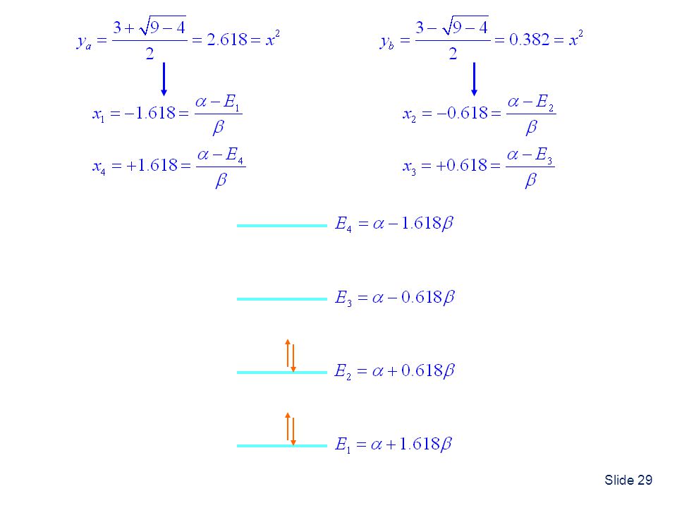
27. Application to Butadiene
1,3-Butadiene has 4  electrons
Note: Application of the Hückel theory to Butadiene is one of your
HW problems.
The solution is worked out in detail below. I will
just outline the solution.
Secular Determinant and Energies
Divide by 
Define

30. Butadiene Delocalization Energy
The additional stabilization of butadiene
compared to 2 ethylenes is a result of
electron delocalization between the
two double bonds.

31. Butadiene Wavefunctions
From first equation:
From second equation:
From fourth equation:

32. Normalization:
(because all overlap integrals are 0)
It is straightforward to perform the same procedure to determine
2 , 3 and 4.
The results are shown on the next slide.

33. C1 C2 C3 C4

34. Butadiene:  Electron Charge and Bond Order
Actually, Butadiene (and the Allyl radical) belong to a class of
hydrocarbons called “Alternant hydrocarbons”, for which all qi = 1.0
All straight-chain polyalkenes are alternant hydrocarbons.

35.  Bond Order:
Note: For a “full”  bond, p = 1.
For a pure  bond, p = 0.
Therefore, the above bond orders reveal that the  bonds between
C1-C2 and C3-C4 are not as strong as in ethylene.
p23 > 0 shows that there is significant  character in the
C2-C3 bond.

36. Part A: The Hückel Model and other Semiempirical Methods
• Hückel Molecular Orbital Model
• Application to Ethylene
• Application to the Allyl Radical (C3H5•)
•  Electron Charge and  Bond Order
• Application to Butadiene
• Introduction of Heteroatoms
• Semiempirical methods for sigma bonded systems

37. Introduction of Heteroatoms
Introduction of a heteroatom such as N or O into a conjugated
system requires different values of  and  than those used for
Carbon because the heteroatom has a different electronegativity;
i.e.Eneg(C) < Eneg(N) <Eneg(O).
It is useful to put the new values of the Coulomb and Resonance Integrals,
X and X (where X is the heteroatom), in terms of the original  and .
The forms that is generally used are:
and
where hX and kX are constants that depend upon the heteroatom.

38. Atom hX
0.5
1.5
2.0
1.0
Bond kX
1.0
0.8
0.4

39. A heteroatom can donate different numbers of electrons into the
 electrons depending upon its bonding.
Example: Nitrogen has 5 valence electrons
In pyridine, 4 of the 5 valence electrons are involved in
2  bonds and (b) 2 electrons in the lone pair.
Therefore, this nitrogen will donate only 1 electron.
In pyrrole, 3 of the electrons will be involved in  bonds.
This nitrogen will donate 2 electrons.

40. Example:  Bonding in Pyrrole
This will illustrate how a heteroatom is handled in the
Hückel Molecular Orbital Model.
For pyrrole, 2 electrons are donated to the  system.
The heteroatom parameters are: hN = 1.5 and kN = 0.8
Therefore:

41. The Secular Determinant

42. This is a 5x5 Secular Determinant, which can be expanded to yield
a fifth order polynomial equation, which can be solved to give:
five values of x.
five energies.
five sets of coefficients.
But, I’m just really not in the mood right now.
Howsabout I just give you the results?
No Applause, PLEASE !!!

43. Wavefunctions and Energies
Note: There are 6 electrons.
Count them.
Note: Actually, I used symmetry to simplify
the 5x5 determinant into a 2x2 and a
3x3 determinant
I’ll show you how at the end of
the chapter.

44.  Electron Charge
 Electron Charge:

45.  Bond Order
 Bond Order:

46. Part A: The Hückel Model and other Semiempirical Methods
• Hückel Molecular Orbital Model
• Application to Ethylene
• Application to the Allyl Radical (C3H5•)
•  Electron Charge and  Bond Order
• Application to Butadiene
• Introduction of Heteroatoms
• Semiempirical methods for sigma bonded systems

47. Semiempirical Methods for Sigma Bonded Systems
The Hückel model was developed to treat only  bond systems.
A number of methods have been developed to treat systems with
 bonded molecules as well as molecules with both  and  bonds.
Three of the most popular are: (1) Pariser-Pople-Parr (PPP) Model
(2) The Extended Hückel model
(3) MNDO methods
We will discuss each method qualitatively.

48. Pariser-Pople-Parr (PPP) Model
The Hückel Model neglects repulsion between electron.
The PPP Model introduces interelectron repulsion into the
effective Hamiltonian:
HPPP = HHückel + HRepulsion
The inclusion of HRepulsion introduces Coulomb Integrals into
the expression for the Energy.
However, these integrals are not calculated.
They are represented by empirical parameters.

49. The Extended Hückel Model
As the title suggests, this is an extension of the Hückel Model to treat
 bonded molecules, developed by Roald Hoffmann (in 1963).
The concept is the same in that one assumes that:
The Molecular Orbitals are linear combinations of atomic
orbitals (i).
2. The total Hamiltonian is a simple sum of effective
one electron Hamiltonians.
3. If one applies the variational principle, then a Secular Determinant
is obtained.

50. • Overlap integrals, Sij are calculated directly (unlike
3. The orbitals for Core shell electrons are ignored. Valence shell
atomic orbitals are given by STOs; e.g. 2s, 2px, 2py, 2pz
4. The parameters in the Secular Determinant are determined
as follows:
• Overlap integrals, Sij are calculated directly (unlike
the Hückel model where they are assumed to be zero)
• Coulomb Integrals, Hii, are set equal to the negative
of the valence shell ionization energies.
• Resonance Integrals, Hij, are calculate with the
Wolfsberg-Helmholtz formula

51. MNDO Methods
An ab initio Hartree-Fock calculation on a molecule requires
the calculation of ~b4/8 integrals.
If one uses a high level basis set on a medium size molecule
(10-20 atoms), a typical number of basis functions might be
b=400, resulting in ~3x109 integrals.
A very great percentage of the time required for a Hartree-Fock
calculation is in the evaluation of these integrals.
There have been a number of semiempirical methods developed
which approximate these integrals. The most popular of these
methods is the MNDO (Modified Neglect of Differential Overlap)
series of methods developed by M. J. S. Dewar.
I’ll comment briefly on them.

52. Assumptions:
Core (inner shell) electrons are not treated explicitly.
An empirical core-core repulsion term is introduced.
A minimal basis set with single ns, npx, npy, npz atomic
orbitals is used to represent valence shell electrons.
Overlap integrals are neglected.
The one-center and two-center integrals are either
ignored or approximated by empirical parameters.
The empirical parameters are obtained by finding the values
that give the best agreement with experimental data;
i.e. Heats of Formation, Ionization Energies, Dipole Moments,etc.

53. The three different MNDO methods are:
MNDO: The original of the methods. In general, this is not
as accurate as later methods.
AM1: This stands for Austin Model 1
Dewar had moved to UT-Austin and wanted to give
credit to his new university.
This method improves upon the parameterization of
the integrals.
PM3: This stands for Parametric Method 3
This improves the parameterization method still further.

54. Because the integrals are determined empirically, and are not
calculated, MNDO methods are thousands of times as fast
as ab initio calculations.
The results are generally not as accurate as ab initio calculations,
but the MNDO methods are good for:
(a) Semi-quantitative results.
(b) Calculations on very large molecules, where
ab initio calculations are not feasible.