1. 4 - 1© 2011 Pearson Education Influence of Product Life Cycle  Introduction and growth require longer forecasts than maturity and decline  As product passes through life cycle, forecasts are useful in projecting  Staffing levels  Inventory levels  Factory capacity Introduction – Growth – Maturity – Decline

2. 4 - 2© 2011 Pearson Education Product Life Cycle Best period to increase market share R&D engineering is critical Practical to change price or quality image Strengthen niche Poor time to change image, price, or quality Competitive costs become critical Defend market position Cost control critical IntroductionGrowthMaturityDecline Company Strategy/Issues Figure 2.5 Internet search engines Sales Drive-through restaurants CD-ROMs Analog TVs iPods Boeing 787 LCD & plasma TVs Twitter Avatars Xbox 360

3. 4 - 3© 2011 Pearson Education Product Life Cycle Product design and development critical Frequent product and process design changes Short production runs High production costs Limited models Attention to quality IntroductionGrowthMaturityDecline OM Strategy/Issues Forecasting critical Product and process reliability Competitive product improvements and options Increase capacity Shift toward product focus Enhance distribution Standardization Fewer product changes, more minor changes Optimum capacity Increasing stability of process Long production runs Product improvement and cost cutting Little product differentiation Cost minimization Overcapacity in the industry Prune line to eliminate items not returning good margin Reduce capacity Figure 2.5

4. 4 - 4© 2011 Pearson Education Types of Forecasts  Economic forecasts  Address business cycle – inflation rate, money supply, housing starts, etc.  Technological forecasts  Predict rate of technological progress  Impacts development of new products  Demand forecasts  Predict sales of existing products and services

5. 4 - 5© 2011 Pearson Education Strategic Importance of Forecasting  Human Resources – Hiring, training, laying off workers  Capacity – Capacity shortages can result in undependable delivery, loss of customers, loss of market share  Supply Chain Management – Good supplier relations and price advantages

6. 4 - 6© 2011 Pearson Education The Realities!  Forecasts are seldom perfect  Most techniques assume an underlying stability in the system  Product family and aggregated forecasts are more accurate than individual product forecasts

7. 4 - 7© 2011 Pearson Education Forecasting Approaches  Used when situation is vague and little data exist  New products  New technology  Involves intuition, experience  e.g., forecasting sales on Internet Qualitative Methods

8. 4 - 8© 2011 Pearson Education Forecasting Approaches  Used when situation is ‘stable’ and historical data exist  Existing products  Current technology  Involves mathematical techniques  e.g., forecasting sales of color televisions Quantitative Methods

9. 4 - 9© 2011 Pearson Education Overview of Qualitative Methods 1.Jury of executive opinion  Pool opinions of high-level experts, sometimes augment by statistical models 2.Delphi method  Panel of experts, queried iteratively

10. 4 - 10© 2011 Pearson Education Overview of Qualitative Methods 3.Sales force composite  Estimates from individual salespersons are reviewed for reasonableness, then aggregated 4.Consumer Market Survey  Ask the customer

11. 4 - 11© 2011 Pearson Education  Involves small group of high-level experts and managers  Group estimates demand by working together  Combines managerial experience with statistical models  Relatively quick  ‘Group-think’ disadvantage Jury of Executive Opinion

12. 4 - 12© 2011 Pearson Education Sales Force Composite  Each salesperson projects his or her sales  Combined at district and national levels  Sales reps know customers’ wants  Tends to be overly optimistic

13. 4 - 13© 2011 Pearson Education Consumer Market Survey  Ask customers about purchasing plans  What consumers say, and what they actually do are often different  Sometimes difficult to answer

14. 4 - 14© 2011 Pearson Education Overview of Quantitative Approaches 1.Naive approach 2.Moving averages 3.Exponential smoothing 4.Trend projection 5.Linear regression time-series models associative model

15. 4 - 15© 2011 Pearson Education Trend Seasonal Cyclical Random Time Series Components

16. 4 - 16© 2011 Pearson Education Components of Demand Demand for product or service |||| 1234 Time (years) Average demand over 4 years Trend component Actual demand line Random variation Figure 4.1 Seasonal peaks

17. 4 - 17© 2011 Pearson Education  Persistent, overall upward or downward pattern  Changes due to population, technology, age, culture, etc.  Typically several years duration Trend Component

18. 4 - 18© 2011 Pearson Education  Regular pattern of up and down fluctuations  Due to weather, customs, etc.  Occurs within a single year Seasonal Component Number of PeriodLengthSeasons WeekDay7 MonthWeek4-4.5 MonthDay28-31 YearQuarter4 YearMonth12 YearWeek52

19. 4 - 19© 2011 Pearson Education  Repeating up and down movements  Affected by business cycle, political, and economic factors  Multiple years duration  Often causal or associative relationships Cyclical Component 05101520

20. 4 - 20© 2011 Pearson Education  Erratic, unsystematic, ‘residual’ fluctuations  Due to random variation or unforeseen events  Short duration and nonrepeating Random Component MTWTFMTWTF

21. 4 - 21© 2011 Pearson Education Naive Approach  Assumes demand in next period is the same as demand in most recent period  e.g., If January sales were 68, then February sales will be 68  Sometimes cost effective and efficient  Can be good starting point

22. 4 - 22© 2011 Pearson Education  MA is a series of arithmetic means  Used if little or no trend  Used often for smoothing  Provides overall impression of data over time Moving Average Method Moving average = ∑ demand in previous n periods n

23. 4 - 23© 2011 Pearson Education January10 February12 March13 April16 May19 June23 July26 Actual3-Month MonthShed SalesMoving Average (12 + 13 + 16)/3 = 13 2 / 3 (13 + 16 + 19)/3 = 16 (16 + 19 + 23)/3 = 19 1 / 3 Moving Average Example 101213 101213 (10 + 12 + 13)/3 = 11 2 / 3

24. 4 - 24© 2011 Pearson Education  Used when some trend might be present  Older data usually less important  Weights based on experience and intuition Weighted Moving Average Weighted moving average = ∑ (weight for period n) x (demand in period n) ∑ weights

25. 4 - 25© 2011 Pearson Education January10 February12 March13 April16 May19 June23 July26 Actual3-Month Weighted MonthShed SalesMoving Average [(3 x 16) + (2 x 13) + (12)]/6 = 14 1 / 3 [(3 x 19) + (2 x 16) + (13)]/6 = 17 [(3 x 23) + (2 x 19) + (16)]/6 = 20 1 / 2 Weighted Moving Average 101213 131210 [(3 x 13) + (2 x 12) + (10)]/6 = 12 1 / 6 Weights AppliedPeriod 3 3Last month 2 2Two months ago 1 1Three months ago 6Sum of weights

26. 4 - 26© 2011 Pearson Education  Form of weighted moving average  Weights decline exponentially  Most recent data weighted most  Requires smoothing constant (  )  Ranges from 0 to 1  Subjectively chosen  Involves little record keeping of past data Exponential Smoothing

27. 4 - 27© 2011 Pearson Education Exponential Smoothing New forecast =Last period’s forecast +  (Last period’s actual demand – Last period’s forecast) F t = F t – 1 +  (A t – 1 - F t – 1 ) whereF t =new forecast F t – 1 =previous forecast  =smoothing (or weighting) constant (0 ≤  ≤ 1)

28. 4 - 28© 2011 Pearson Education Exponential Smoothing Example Predicted demand = 142 Ford Mustangs Actual demand = 153 Smoothing constant  =.20

29. 4 - 29© 2011 Pearson Education Exponential Smoothing Example Predicted demand = 142 Ford Mustangs Actual demand = 153 Smoothing constant  =.20 New forecast= 142 +.2(153 – 142)

30. 4 - 30© 2011 Pearson Education Exponential Smoothing Example Predicted demand = 142 Ford Mustangs Actual demand = 153 Smoothing constant  =.20 New forecast= 142 +.2(153 – 142) = 142 + 2.2 = 144.2 ≈ 144 cars

31. 4 - 31© 2011 Pearson Education Choosing  The objective is to obtain the most accurate forecast no matter the technique We generally do this by selecting the model that gives us the lowest forecast error Forecast error= Actual demand - Forecast value = A t - F t

32. 4 - 32© 2011 Pearson Education Common Measures of Error Mean Absolute Deviation (MAD) MAD = ∑ |Actual - Forecast| n Mean Squared Error (MSE) MSE = ∑ (Forecast Errors) 2 n

33. 4 - 33© 2011 Pearson Education Common Measures of Error Mean Absolute Percent Error (MAPE) MAPE = ∑ 100|Actual i - Forecast i |/Actual i n i = 1

34. 4 - 34© 2011 Pearson Education Comparison of Forecast Error RoundedAbsoluteRoundedAbsolute ActualForecastDeviationForecastDeviation Tonnagewithforwithfor QuarterUnloaded  =.10  =.10  =.50  =.50 11801755.001755.00 2168175.57.50177.509.50 3159174.7515.75172.7513.75 4175173.181.82165.889.12 5190173.3616.64170.4419.56 6205175.0229.98180.2224.78 7180178.021.98192.6112.61 8182178.223.78186.304.30 82.4598.62

35. 4 - 35© 2011 Pearson Education Comparison of Forecast Error RoundedAbsoluteRoundedAbsolute ActualForecastDeviationForecastDeviation Tonnagewithforwithfor QuarterUnloaded  =.10  =.10  =.50  =.50 11801755.001755.00 2168175.57.50177.509.50 3159174.7515.75172.7513.75 4175173.181.82165.889.12 5190173.3616.64170.4419.56 6205175.0229.98180.2224.78 7180178.021.98192.6112.61 8182178.223.78186.304.30 82.4598.62 MAD = ∑ |deviations| n = 82.45/8 = 10.31 For  =.10 = 98.62/8 = 12.33 For  =.50

36. 4 - 36© 2011 Pearson Education Comparison of Forecast Error RoundedAbsoluteRoundedAbsolute ActualForecastDeviationForecastDeviation Tonnagewithforwithfor QuarterUnloaded  =.10  =.10  =.50  =.50 11801755.001755.00 2168175.57.50177.509.50 3159174.7515.75172.7513.75 4175173.181.82165.889.12 5190173.3616.64170.4419.56 6205175.0229.98180.2224.78 7180178.021.98192.6112.61 8182178.223.78186.304.30 82.4598.62 MAD10.3112.33 = 1,526.54/8 = 190.82 For  =.10 = 1,561.91/8 = 195.24 For  =.50 MSE = ∑ (forecast errors) 2 n

37. 4 - 37© 2011 Pearson Education Comparison of Forecast Error RoundedAbsoluteRoundedAbsolute ActualForecastDeviationForecastDeviation Tonnagewithforwithfor QuarterUnloaded  =.10  =.10  =.50  =.50 11801755.001755.00 2168175.57.50177.509.50 3159174.7515.75172.7513.75 4175173.181.82165.889.12 5190173.3616.64170.4419.56 6205175.0229.98180.2224.78 7180178.021.98192.6112.61 8182178.223.78186.304.30 82.4598.62 MAD10.3112.33 MSE190.82195.24 = 44.75/8 = 5.59% For  =.10 = 54.05/8 = 6.76% For  =.50 MAPE = ∑ 100|deviation i |/actual i n i = 1

38. 4 - 38© 2011 Pearson Education Comparison of Forecast Error RoundedAbsoluteRoundedAbsolute ActualForecastDeviationForecastDeviation Tonnagewithforwithfor QuarterUnloaded  =.10  =.10  =.50  =.50 11801755.001755.00 2168175.57.50177.509.50 3159174.7515.75172.7513.75 4175173.181.82165.889.12 5190173.3616.64170.4419.56 6205175.0229.98180.2224.78 7180178.021.98192.6112.61 8182178.223.78186.304.30 82.4598.62 MAD10.3112.33 MSE190.82195.24 MAPE5.59%6.76%

39. 4 - 39© 2011 Pearson Education Trend Projections Fitting a trend line to historical data points to project into the medium to long-range Linear trends can be found using the least squares technique y = a + bx ^ where y= computed value of the variable to be predicted (dependent variable) a= y-axis intercept b= slope of the regression line x= the independent variable ^

40. 4 - 40© 2011 Pearson Education Least Squares Method Equations to calculate the regression variables b =  xy - nxy  x 2 - nx 2 y = a + bx ^ a = y - bx

41. 4 - 41© 2011 Pearson Education Least Squares Example b = = = 10.54 ∑xy - nxy ∑x 2 - nx 2 3,063 - (7)(4)(98.86) 140 - (7)(4 2 ) a = y - bx = 98.86 - 10.54(4) = 56.70 TimeElectrical Power YearPeriod (x)Demandx 2 xy 2003174174 20042794158 20053809240 200649016360 2007510525525 2008614236852 2009712249854 ∑x = 28∑y = 692∑x 2 = 140∑xy = 3,063 x = 4y = 98.86

42. 4 - 42© 2011 Pearson Education b = = = 10.54 ∑xy - nxy ∑x 2 - nx 2 3,063 - (7)(4)(98.86) 140 - (7)(4 2 ) a = y - bx = 98.86 - 10.54(4) = 56.70 TimeElectrical Power YearPeriod (x)Demandx 2 xy 2003174174 20042794158 20053809240 200649016360 2007510525525 2008614236852 2009712249854 ∑x = 28∑y = 692∑x 2 = 140∑xy = 3,063 x = 4y = 98.86 Least Squares Example The trend line is y = 56.70 + 10.54x ^

43. 4 - 43© 2011 Pearson Education Least Squares Example ||||||||| 200320042005200620072008200920102011 160 – 150 – 140 – 130 – 120 – 110 – 100 – 90 – 80 – 70 – 60 – 50 – Year Power demand Trend line, y = 56.70 + 10.54x ^

44. 4 - 44© 2011 Pearson Education Least Squares Requirements 1.We always plot the data to insure a linear relationship 2.We do not predict time periods far beyond the database 3.Deviations around the least squares line are assumed to be random

45. 4 - 45© 2011 Pearson Education Seasonal Variations In Data The multiplicative seasonal model can adjust trend data for seasonal variations in demand

46. 4 - 46© 2011 Pearson Education Seasonal Variations In Data 1.Find average historical demand for each season 2.Compute the average demand over all seasons 3.Compute a seasonal index for each season 4.Estimate next year’s total demand 5.Divide this estimate of total demand by the number of seasons, then multiply it by the seasonal index for that season Steps in the process:

47. 4 - 47© 2011 Pearson Education Seasonal Index Example Jan80851059094 Feb7085858094 Mar8093828594 Apr909511510094 May11312513112394 Jun11011512011594 Jul10010211310594 Aug8810211010094 Sept8590959094 Oct7778858094 Nov7572838094 Dec8278808094 DemandAverageAverage Seasonal Month2007200820092007-2009MonthlyIndex

48. 4 - 48© 2011 Pearson Education Seasonal Index Example Jan80851059094 Feb7085858094 Mar8093828594 Apr909511510094 May11312513112394 Jun11011512011594 Jul10010211310594 Aug8810211010094 Sept8590959094 Oct7778858094 Nov7572838094 Dec8278808094 DemandAverageAverage Seasonal Month2007200820092007-2009MonthlyIndex 0.957 Seasonal index = Average 2007-2009 monthly demand Average monthly demand = 90/94 =.957

49. 4 - 49© 2011 Pearson Education Seasonal Index Example Jan808510590940.957 Feb70858580940.851 Mar80938285940.904 Apr9095115100941.064 May113125131123941.309 Jun110115120115941.223 Jul100102113105941.117 Aug88102110100941.064 Sept85909590940.957 Oct77788580940.851 Nov75728380940.851 Dec82788080940.851 DemandAverageAverage Seasonal Month2007200820092007-2009MonthlyIndex

50. 4 - 50© 2011 Pearson Education Seasonal Index Example Jan808510590940.957 Feb70858580940.851 Mar80938285940.904 Apr9095115100941.064 May113125131123941.309 Jun110115120115941.223 Jul100102113105941.117 Aug88102110100941.064 Sept85909590940.957 Oct77788580940.851 Nov75728380940.851 Dec82788080940.851 DemandAverageAverage Seasonal Month2007200820092007-2009MonthlyIndex Expected annual demand = 1,200 Janx.957 = 96 1,200 12 Febx.851 = 85 1,200 12 Forecast for 2010

51. 4 - 51© 2011 Pearson Education Seasonal Index Example 140 – 130 – 120 – 110 – 100 – 90 – 80 – 70 – ||||||||||||JFMAMJJASOND||||||||||||JFMAMJJASOND Time Demand 2010 Forecast 2009 Demand 2008 Demand 2007 Demand

52. 4 - 52© 2011 Pearson Education Associative Forecasting Used when changes in one or more independent variables can be used to predict the changes in the dependent variable Most common technique is linear regression analysis We apply this technique just as we did in the time series example

53. 4 - 53© 2011 Pearson Education Associative Forecasting Forecasting an outcome based on predictor variables using the least squares technique y = a + bx ^ where y= computed value of the variable to be predicted (dependent variable) a= y-axis intercept b= slope of the regression line x= the independent variable though to predict the value of the dependent variable ^

54. 4 - 54© 2011 Pearson Education Associative Forecasting Example SalesArea Payroll ($ millions), y($ billions), x 2.01 3.03 2.54 2.02 2.01 3.57 4.0 – 3.0 – 2.0 – 1.0 – |||||||01234567|||||||01234567 Sales Area payroll

55. 4 - 55© 2011 Pearson Education Associative Forecasting Example Sales, y Payroll, xx 2 xy 2.0112.0 3.0399.0 2.541610.0 2.0244.0 2.0112.0 3.574924.5 ∑y = 15.0∑x = 18∑x 2 = 80∑xy = 51.5 x = ∑x/6 = 18/6 = 3 y = ∑y/6 = 15/6 = 2.5 b = = =.25 ∑xy - nxy ∑x 2 - nx 2 51.5 - (6)(3)(2.5) 80 - (6)(3 2 ) a = y - bx = 2.5 - (.25)(3) = 1.75

56. 4 - 56© 2011 Pearson Education Associative Forecasting Example y = 1.75 +.25x ^ Sales = 1.75 +.25(payroll) If payroll next year is estimated to be $6 billion, then: Sales = 1.75 +.25(6) Sales = $3,250,000 4.0 – 3.0 – 2.0 – 1.0 – |||||||01234567|||||||01234567 Nodel’s sales Area payroll 3.25

57. 4 - 57© 2011 Pearson Education  How strong is the linear relationship between the variables?  Correlation does not necessarily imply causality!  Coefficient of correlation, r, measures degree of association  Values range from -1 to +1 Correlation

58. 4 - 58© 2011 Pearson Education Correlation Coefficient r = n  xy -  x  y [n  x 2 - (  x) 2 ][n  y 2 - (  y) 2 ]

59. 4 - 59© 2011 Pearson Education Correlation Coefficient r = n  xy -  x  y [n  x 2 - (  x) 2 ][n  y 2 - (  y) 2 ] y x (a)Perfect positive correlation: r = +1 y x (b)Positive correlation: 0 < r < 1 y x (c)No correlation: r = 0 y x (d)Perfect negative correlation: r = -1

60. 4 - 60© 2011 Pearson Education  Coefficient of Determination, r 2, measures the percent of change in y predicted by the change in x  Values range from 0 to 1  Easy to interpret Correlation For the Nodel Construction example: r =.901 r 2 =.81

61. 4 - 61© 2011 Pearson Education Adaptive Forecasting  It’s possible to use the computer to continually monitor forecast error and adjust the values of the  and  coefficients used in exponential smoothing to continually minimize forecast error  This technique is called adaptive smoothing

62. 4 - 62© 2011 Pearson Education Focus Forecasting  Developed at American Hardware Supply, based on two principles: 1.Sophisticated forecasting models are not always better than simple ones 2.There is no single technique that should be used for all products or services  This approach uses historical data to test multiple forecasting models for individual items  The forecasting model with the lowest error is then used to forecast the next demand

63. 4 - 63© 2011 Pearson Education Forecasting in the Service Sector  Presents unusual challenges  Special need for short term records  Needs differ greatly as function of industry and product  Holidays and other calendar events  Unusual events

64. 4 - 64© 2011 Pearson Education Fast Food Restaurant Forecast 20% – 15% – 10% – 5% – 11-121-23-45-67-89-10 12-12-34-56-78-910-11 (Lunchtime)(Dinnertime) Hour of day Percentage of sales Figure 4.12

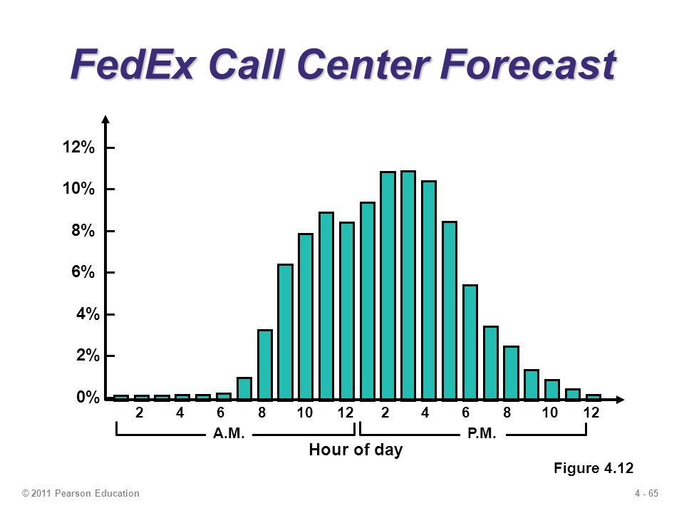
65. 4 - 65© 2011 Pearson Education FedEx Call Center Forecast Figure 4.12 12% – 10% – 8% – 6% – 4% – 2% – 0% – Hour of day A.M.P.M. 2468101224681012