Download presentation
Presentation is loading. Please wait.

1
High Throughput Sequencing
Xiaole Shirley Liu STAT115, STAT215, BIO298, BIST520 Guest lecturer: Wei Li

2
About me Wei Li, research fellow at DFCI
Studied high-throughput sequencing algorithms shortly after HTS comes out (2009) Transcript reconstruction algorithms from high-throughput RNA sequencing data (RNA-seq): IsoInfer/IsoLasso/CEM CRISPR/Cas9 screening algorithms: design, analysis (MAGeCK/MAGeCK-VISPR)
 Transcript reconstruction algorithms from high-throughput RNA sequencing data (RNA-seq): IsoInfer/IsoLasso/CEM. CRISPR/Cas9 screening algorithms: design, analysis (MAGeCK/MAGeCK-VISPR)")
3
Why high-throughput sequencing?
High-throughput sequencing/HTS/Next-generation sequencing/NGS 2-3 orders of magnitude faster/cheaper/higher data throughput compared with “first generation” Huge applications in academia/industry

4
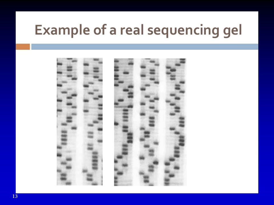
First generation: Sanger sequencing
Frederick Sanger: the 3rd person overall to win two Nobel prizes

5
First Generation Sanger Sequencing: 384 * 1kb / 3 hours

6
Sanger sequencing materials
Sanger sequencing uses DNA elongation to “read” sequences dNTPs: required for normal elongation process ddNTPs: missing oxygen bond, will stop the synthesis dideoxyNTP, di=two, deoxy=remove oxygen

7
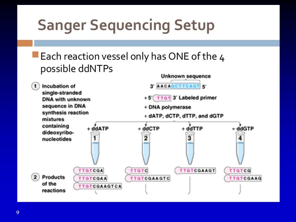
Sanger sequencing setup
4 tubes, each test tube has deoxyA,G,C,T In addition each also has ONE of the 4 ddNTP

8
What happens if you have both dATP and ddATP?
The synthesis stops whenever you encounter “T”

14
Sequencing in 2001 [Enter any extra notes here; leave the item ID line at the bottom] Avitage Item ID: {{CE8AAEAA-A22F-47FE-A1F8-66CBC3CDB6FC}}
![Sequencing in 2001 [Enter any extra notes here; leave the item ID line at the bottom] Avitage Item ID: {{CE8AAEAA-A22F-47FE-A1F8-66CBC3CDB6FC}}](http://slideplayer.com/slide/10965296/39/images/14/Sequencing+in+2001+%5BEnter+any+extra+notes+here%3B+leave+the+item+ID+line+at+the+bottom%5D+Avitage+Item+ID%3A+%7B%7BCE8AAEAA-A22F-47FE-A1F8-66CBC3CDB6FC%7D%7D.jpg "Sequencing in 2001 [Enter any extra notes here; leave the item ID line at the bottom] Avitage Item ID: {{CE8AAEAA-A22F-47FE-A1F8-66CBC3CDB6FC}}")
15
Sequencing in 2007 [Enter any extra notes here; leave the item ID line at the bottom] Avitage Item ID: {{010D7619-E070-4F7B-BC AA639C8D}}
![Sequencing in 2007 [Enter any extra notes here; leave the item ID line at the bottom] Avitage Item ID: {{010D7619-E070-4F7B-BC AA639C8D}}](http://slideplayer.com/slide/10965296/39/images/15/Sequencing+in+2007+%5BEnter+any+extra+notes+here%3B+leave+the+item+ID+line+at+the+bottom%5D+Avitage+Item+ID%3A+%7B%7B010D7619-E070-4F7B-BC+AA639C8D%7D%7D.jpg "Sequencing in 2007 [Enter any extra notes here; leave the item ID line at the bottom] Avitage Item ID: {{010D7619-E070-4F7B-BC AA639C8D}}")
16
Second Generation Massively parallel sequencing by synthesis
Many different technologies: Illumina, 454, SOLiD, Helicos, etc Illumina: HiSeq, MiSeq, NextSeq 1-16 samples 25M-4B reads 30-300bp 1-8 days 15GB-1TB output Moving targets

17
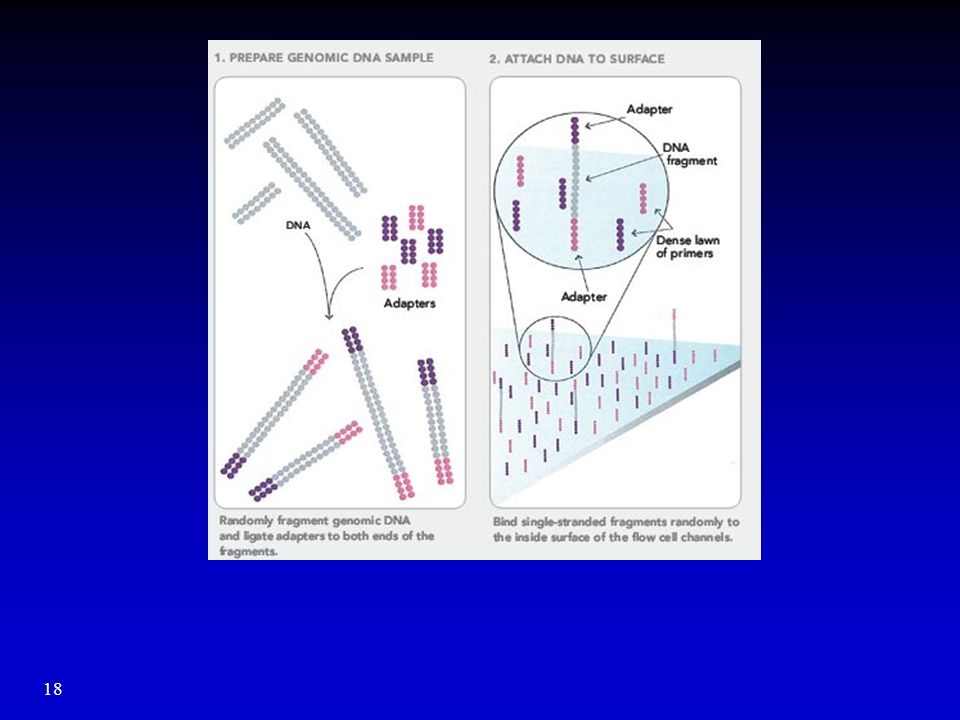
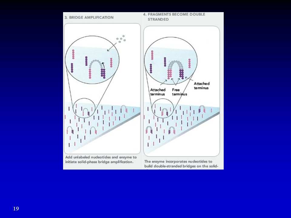
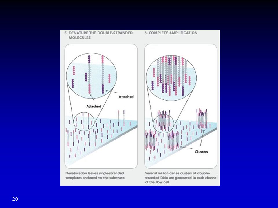
Illumina Cluster Generation
Amplify sequenced fragments in place on the flow cell Can sequence from both the pink and purple adapters (Paired-end seq) Can multiplex many samples / lane
 Can multiplex many samples / lane.")
21
Illumina Sequencing process
1. Incorporate all 4 nucleotides, each label with a different dye 2. Wash, 4-color imaging 4. Repeat cycles 3. Cleave dye and terminating groups, wash

22
Illumina Sequencing Cycle 1 2 3 4 5 6

23
Third Generation Single molecule sequencing: no amp
Fewer but much longer reads Good for sequencing long reads, but not for read count applications, technology still in developmenthttp://

24
High Throughput Sequencing
Big (data), fast (speed), cheap (cost), flexible (applications) Cost reduces faster than Moore’s law: Bioinformatic analyses become bottleneck!
, fast (speed), cheap (cost), flexible (applications) Cost reduces faster than Moore’s law: Bioinformatic analyses become bottleneck!")
25
High Throughput Sequencing Data Analysis

26
FASTQ File Format Quality score using ASCII (higher -> better)
Sequence ID, sequence Quality ID, quality score Quality score using ASCII (higher -> better) @HWI-EAS305:1:1:1:991#0/1 GCTGGAGGTTCAGGCTGGCCGGATTTAAACGTAT +HWI-EAS305:1:1:1:991#0/1 MVXUWVRKTWWULRQQMMWWBBBBBBBBBBBBBB @HWI-EAS305:1:1:1:201#0/1 AAGACAAAGATGTGCTTTCTAAATCTGCACTAAT +HWI-EAS305:1:1:1:201#0/1 PXX[[[[XTXYXTTWYYY[XXWWW[TMTVXWBBB

27
FASTQC: Sequencing Quality
Good quality! Poor quality!

28
Read Mapping Mapping hundreds of millions of reads back to the reference genome is CPU and RAM intensive and slow Read quality decreases with length (small single nucleotide mismatches or indels) Most mappers allow ~2 mismatches within first 30bp (4 ^ 28 could still uniquely identify most 30bp sequences in a 3GB genome), slower when allowing indels Mapping output: SAM (BAM) or BED
 Most mappers allow ~2 mismatches within first 30bp (4 ^ 28 could still uniquely identify most 30bp sequences in a 3GB genome), slower when allowing indels. Mapping output: SAM (BAM) or BED.")
29
Read mapping algorithms
Spaced seed alignment Burrows-Wheeler Suffix tree

30
Spaced seed alignment Tags and tag-sized pieces of reference are cut into small “seeds.” Pairs of spaced seeds are stored in an index. Look up spaced seeds for each tag. For each “hit,” confirm the remaining positions. Report results to the user.

31
BW alignment

32
Burrows-Wheeler Store entire reference genome.
Align tag base by base from the end. When tag is traversed, all active locations are reported. If no match is found, then back up and try a substitution. Trapnell & Salzberg, Nat Biotech 2009

33
Burrows-Wheeler Transform
Reversible permutation used originally in compression Once BWT(T) is built, all else shown here is discarded First col can be derived by sorting the last col T (query sequence) BWT(T) Encoding for compression gc$ac Burrows Wheeler Matrix Last column Burrows M, Wheeler DJ: A block sorting lossless data compression algorithm. Digital Equipment Corporation, Palo Alto, CA 1994, Technical Report 124; 1994 Slides from Ben Langmead
 is built, all else shown here is discarded. First col can be derived by sorting the last col. T. (query sequence) BWT(T) Encoding for. compression. gc$ac Burrows. Wheeler. Matrix. Last column. Burrows M, Wheeler DJ: A block sorting lossless data compression algorithm. Digital Equipment Corporation, Palo Alto, CA 1994, Technical Report 124; Slides from Ben Langmead.")
34
Burrows-Wheeler Transform
Property that makes BWT(T) reversible is “LF Mapping” ith occurrence of a character in Last column is same text occurrence as the ith occurrence in First column Rank: 2 (2nd ‘a’ in First column) BWT(T) T Rank: 2 (2nd ‘a’ in Last column) Burrows Wheeler Matrix Slides modified from Ben Langmead
 reversible is LF Mapping ith occurrence of a character in Last column is same text occurrence as the ith occurrence in First column. Rank: 2. (2nd ‘a’ in First column) BWT(T) T. Rank: 2. (2nd ‘a’ in Last column) Burrows Wheeler. Matrix. Slides modified from Ben Langmead.")
35
BWT: How to reconstruct T from BWT(T)?
To recreate T from BWT(T), repeatedly apply rule: T = BWT[ LF(i) ] + T; i = LF(i) Where LF(i) maps row i to row whose first character corresponds to i’s last per LF Mapping Final T Slides from Ben Langmead
, repeatedly apply rule: T = BWT[ LF(i) ] + T; i = LF(i) Where LF(i) maps row i to row whose first character corresponds to i’s last per LF Mapping. Final T. Slides from Ben Langmead.")
36
BWT: How to reconstruct T from BWT(T)?
To recreate T from BWT(T), repeatedly apply rule: T = BWT[ LF(i) ] + T; i = LF(i) Where LF(i) maps row i to row whose first character corresponds to i’s last per LF Mapping LF(i)=7; the first ‘g’ BWT[LF(i)]=‘c’; the second last character is ‘c’; i=LF(i)=7 i=1; this is the last character of T The first and last columns are known Slides from Ben Langmead
, repeatedly apply rule: T = BWT[ LF(i) ] + T; i = LF(i) Where LF(i) maps row i to row whose first character corresponds to i’s last per LF Mapping. LF(i)=7; the first ‘g’ BWT[LF(i)]=‘c’; the second last character is ‘c’; i=LF(i)=7. i=1; this is the last character of T. The first and last columns are known. Slides from Ben Langmead.")
37
BWT: How to reconstruct T from BWT(T)?
To recreate T from BWT(T), repeatedly apply rule: T = BWT[ LF(i) ] + T; i = LF(i) Where LF(i) maps row i to row whose first character corresponds to i’s last per LF Mapping LF(i)=6; the second ‘c’ BWT[LF(i)]=‘a’; the 3rd last character is a’; i=LF(i)=6 i=7; this is the second last character of T Slides from Ben Langmead
, repeatedly apply rule: T = BWT[ LF(i) ] + T; i = LF(i) Where LF(i) maps row i to row whose first character corresponds to i’s last per LF Mapping. LF(i)=6; the second ‘c’ BWT[LF(i)]=‘a’; the 3rd last character is a’; i=LF(i)=6. i=7; this is the second last character of T. Slides from Ben Langmead.")
38
BWT: How to reconstruct T from BWT(T)?
To recreate T from BWT(T), repeatedly apply rule: T = BWT[ LF(i) ] + T; i = LF(i) Where LF(i) maps row i to row whose first character corresponds to i’s last per LF Mapping Final T Slides from Ben Langmead
, repeatedly apply rule: T = BWT[ LF(i) ] + T; i = LF(i) Where LF(i) maps row i to row whose first character corresponds to i’s last per LF Mapping. Final T. Slides from Ben Langmead.")
39
BWT: How To Do Exact Matching?
To match Q in T using BWT(T), repeatedly apply rule: top = LF(top, qc); bot = LF(bot, qc) Where qc is the next character in Q (right-to-left) and LF(i, qc) maps row i to the row whose first character corresponds to i’s last character as if it were qc Slides from Ben Langmead
, repeatedly apply rule: top = LF(top, qc); bot = LF(bot, qc) Where qc is the next character in Q (right-to-left) and LF(i, qc) maps row i to the row whose first character corresponds to i’s last character as if it were qc. Slides from Ben Langmead.")
40
BWT: How To Do Exact Matching?
To match Q in T using BWT(T), repeatedly apply rule: top = LF(top, qc); bot = LF(bot, qc) Where qc is the next character in Q (right-to-left) and LF(i, qc) maps row i to the row whose first character corresponds to i’s last character as if it were qc qc=‘a’ top=LF(5,’a’)=3 bot=LF(6,’a’)=4 qc=‘c’ top=5 The last character of row 5,6 is ‘a’ bot=6 Slides from Ben Langmead
, repeatedly apply rule: top = LF(top, qc); bot = LF(bot, qc) Where qc is the next character in Q (right-to-left) and LF(i, qc) maps row i to the row whose first character corresponds to i’s last character as if it were qc. qc=‘a’ top=LF(5,’a’)=3. bot=LF(6,’a’)=4. qc=‘c’ top=5. The last character of row 5,6 is ‘a’ bot=6. Slides from Ben Langmead.")
41
BWT: How To Do Exact Matching?
To match Q in T using BWT(T), repeatedly apply rule: top = LF(top, qc); bot = LF(bot, qc) Where qc is the next character in Q (right-to-left) and LF(i, qc) maps row i to the row whose first character corresponds to i’s last character as if it were qc qc=‘a’ top=LF(3,’a’)=2 bot=LF(4,’a’)=2 The last character of row 3,4 is ‘a’,’$’ Slides from Ben Langmead
, repeatedly apply rule: top = LF(top, qc); bot = LF(bot, qc) Where qc is the next character in Q (right-to-left) and LF(i, qc) maps row i to the row whose first character corresponds to i’s last character as if it were qc. qc=‘a’ top=LF(3,’a’)=2. bot=LF(4,’a’)=2. The last character of row 3,4 is ‘a’,’$’ Slides from Ben Langmead.")
42
Exact Matching with FM Index
In progressive rounds, top & bot delimit the range of rows beginning with progressively longer suffixes of Q (from right to left) If range becomes empty the query suffix (and therefore the query) does not occur in the text If no match, instead of giving up, try to “backtrack” to a previous position and try a different base (mismatch, much slower) Slides from Ben Langmead
 If range becomes empty the query suffix (and therefore the query) does not occur in the text. If no match, instead of giving up, try to backtrack to a previous position and try a different base (mismatch, much slower) Slides from Ben Langmead.")
43
STAR Alignment Suffix Tree
Very fast and accuracy for mapping PE-seq and high read counts O(n) time to build O(mlogn) time to search
 time to build. O(mlogn) time to. search.")
44
Suffix tree (Example) Let s=abab, a suffix tree of s is a compressed trie of all suffixes of s=abab$ $ { $ b$ ab$ bab$ abab$ } a b $

45
Mapped Seq Files Mapped SAM
HWUSI-EAS366_0112:6:1:1298:18828#0/1 16 chr9 255 38M * 0 0 TACAATATGTCTTTATTTGAGATATGGATTTTAGGCCG Y\]bc^dab\[_UU`^`LbTUT\ccLbbYaY`cWLYW^ XA:i:1 MD:Z:3C30T3 NM:i:2 HWUSI-EAS366_0112:6:1:1257:18819#0/1 4 * 0 0 * * 0 0 AGACCACATGAAGCTCAAGAAGAAGGAAGACAAAAGTG ece^dddT\cT^c`a`ccdK\c^^__]Yb\_cKS^_W\ XM:i:1 HWUSI-EAS366_0112:6:1:1315:19529#0/1 16 chr9 255 38M * 0 0 GCACTCAAGGGTACAGGAAAAGGGTCAGAAGTGTGGCC ^c_Yc\Lcb`bbYdTa\dd\`dda`cdd\Y\ddd^cT` XA:i:0 MD:Z:38 NM:i:0 chr chr Mapped SAM Map: 0 OK, 4 unmapped, 16 mapped reverse strand Sequence, quality score XA (mapper-specific) MD: mismatch info: 3 match, then C ref, 30 match, then T ref, 3 match NM: number of mismatch BAM: binary SAM format Mapped BED Chr, start, end, strand
 MD: mismatch info: 3 match, then C ref, 30 match, then T ref, 3 match. NM: number of mismatch. BAM: binary SAM format. Mapped BED. Chr, start, end, strand.")
46
Mapping Statistics Terms
Mappable locations: reads that can find match to A location in the genome Uniquely mapped reads: reads that can find match to A SINGLE location in the genome Repeat sequences in the genome, length-dependent Uniquely mapped locations: number of unique locations hit by uniquely mapped reads Redundancy: potential PCR amplification bias

47
Summary Sequencing technologies Sequence quality assessment
1st, 2nd, 3rd generation Sequence quality assessment FASTQC Read mapping Spaced seed BWA: Borrows Wheeler transformation, LF mapping STAR: Suffix Tree, fast SAM / BAM format

Similar presentations
 A2 is online We considered the basics of sequence alignment –Opt score.>")


 Isolate total RNA Isolate mRNA from total RNA (poly.>")


