1. CS558 C OMPUTER V ISION Lecture IV: Image Filter and Edge Detection Slides adapted from S. Lazebnik

2. R ECAP OF L ECTURE III Light and Shade Radiance and irradiance Radiometry of thin lens Bidirectional reflectance distribution function (BRDF) Photometric stereo Color What is color? Human eyes Trichromacy and color space Color perception

3. O UTLINE Image filter and convolution Convluation and linear filter Gaussian filter, box filter, and median filter Application: Hybrid images Edge detection Image derivatives Gaussian derivative filters Canny edge detector

4. O UTLINE Image filter and convolution Convolution and linear filter Gaussian filter, box filter, and median filter Application: Hybrid images Edge detection Image derivatives Gaussian derivative filters Canny edge detector

5. M OTIVATION : I MAGE DENOISING How can we reduce noise in a photograph?

6. M OVING AVERAGE Let’s replace each pixel with a weighted average of its neighborhood The weights are called the filter kernel What are the weights for the average of a 3x3 neighborhood? 111 111 111 “box filter” Source: D. Lowe

7. O UTLINE Image filter and convolution Convolution and linear filter Gaussian filter, box filter, and median filter Application: Hybrid images Edge detection Image derivatives Gaussian derivative filters Canny edge detector

8. D EFINING CONVOLUTION Let f be the image and g be the kernel. The output of convolving f with g is denoted f * g. f Source: F. Durand MATLAB functions: conv2, filter2, imfilter

9. K EY PROPERTIES Linearity: filter( f 1 + f 2 ) = filter( f 1 ) + filter( f 2 ) Shift invariance: same behavior regardless of pixel location: filter(shift( f )) = shift(filter( f )) Theoretical result: any linear shift-invariant operator can be represented as a convolution

10. P ROPERTIES IN MORE DETAIL Commutative: a * b = b * a Conceptually no difference between filter and signal Associative: a * ( b * c ) = ( a * b ) * c Often apply several filters one after another: ((( a * b 1 ) * b 2 ) * b 3 ) This is equivalent to applying one filter: a * ( b 1 * b 2 * b 3 ) Distributes over addition: a * ( b + c ) = ( a * b ) + ( a * c ) Scalars factor out: ka * b = a * kb = k ( a * b ) Identity: unit impulse e = […, 0, 0, 1, 0, 0, …], a * e = a

11. A NNOYING DETAILS What is the size of the output? MATLAB: filter2(g, f, shape ) shape = ‘full’: output size is sum of sizes of f and g shape = ‘same’: output size is same as f shape = ‘valid’: output size is difference of sizes of f and g f gg gg f gg g g f gg gg full samevalid

12. A NNOYING DETAILS What about near the edge? the filter window falls off the edge of the image need to extrapolate methods: clip filter (black) wrap around copy edge reflect across edge Source: S. Marschner

13. A NNOYING DETAILS What about near the edge? the filter window falls off the edge of the image need to extrapolate methods (MATLAB): clip filter (black): imfilter(f, g, 0) wrap around:imfilter(f, g, ‘circular’) copy edge: imfilter(f, g, ‘replicate’) reflect across edge: imfilter(f, g, ‘symmetric’) Source: S. Marschner

14. P RACTICE WITH LINEAR FILTERS 000 010 000 Original ? Source: D. Lowe

15. P RACTICE WITH LINEAR FILTERS 000 010 000 Original Filtered (no change) Source: D. Lowe

16. P RACTICE WITH LINEAR FILTERS 000 100 000 Original ? Source: D. Lowe

17. P RACTICE WITH LINEAR FILTERS 000 100 000 Original Shifted left By 1 pixel Source: D. Lowe

18. P RACTICE WITH LINEAR FILTERS Original ? 111 111 111 Source: D. Lowe

19. P RACTICE WITH LINEAR FILTERS Original 111 111 111 Blur (with a box filter) Source: D. Lowe

20. P RACTICE WITH LINEAR FILTERS Original 111 111 111 000 020 000 - ? (Note that filter sums to 1) Source: D. Lowe

21. P RACTICE WITH LINEAR FILTERS Original 111 111 111 000 020 000 - Sharpening filter - Accentuates differences with local average Source: D. Lowe

22. S HARPENING Source: D. Lowe

23. S HARPENING What does blurring take away? original smoothed (5x5) – detail = sharpened = Let’s add it back: originaldetail +

24. S MOOTHING WITH BOX FILTER REVISITED What’s wrong with this picture? What’s the solution? Source: D. Forsyth

25. S MOOTHING WITH BOX FILTER REVISITED What’s wrong with this picture? What’s the solution? To eliminate edge effects, weight contribution of neighborhood pixels according to their closeness to the center “fuzzy blob”

26. O UTLINE Image filter and convolution Convluation and linear filter Gaussian filter, box filter, and median filter Application: Hybrid images Edge detection Image derivatives Gaussian derivative filters Canny edge detector

27. G AUSSIAN K ERNEL Constant factor at front makes volume sum to 1 (can be ignored when computing the filter values, as we should renormalize weights to sum to 1 in any case) 0.003 0.013 0.022 0.013 0.003 0.013 0.059 0.097 0.059 0.013 0.022 0.097 0.159 0.097 0.022 0.013 0.059 0.097 0.059 0.013 0.003 0.013 0.022 0.013 0.003 5 x 5,  = 1 Source: C. Rasmussen

28. G AUSSIAN K ERNEL Standard deviation  : determines extent of smoothing Source: K. Grauman σ = 2 with 30 x 30 kernel σ = 5 with 30 x 30 kernel

29. C HOOSING KERNEL WIDTH The Gaussian function has infinite support, but discrete filters use finite kernels Source: K. Grauman

30. C HOOSING KERNEL WIDTH Rule of thumb: set filter half-width to about 3 σ

31. G AUSSIAN VS. BOX FILTERING

32. G AUSSIAN FILTERS Remove “high-frequency” components from the image (low-pass filter) Convolution with self is another Gaussian So can smooth with small-  kernel, repeat, and get same result as larger-  kernel would have Convolving two times with Gaussian kernel with std. dev. σ is same as convolving once with kernel with std. dev. Separable kernel Factors into product of two 1D Gaussians Source: K. Grauman

33. S EPARABILITY OF THE G AUSSIAN FILTER Source: D. Lowe

34. S EPARABILITY EXAMPLE * * = = 2D convolution (center location only) Source: K. Grauman The filter factors into a product of 1D filters: Perform convolution along rows: Followed by convolution along the remaining column:

35. W HY IS SEPARABILITY USEFUL ? What is the complexity of filtering an n × n image with an m × m kernel? O(n 2 m 2 ) What if the kernel is separable? O(n 2 m)

36. N OISE Salt and pepper noise : contains random occurrences of black and white pixels Impulse noise: contains random occurrences of white pixels Gaussian noise : variations in intensity drawn from a Gaussian normal distribution Source: S. Seitz

37. G AUSSIAN NOISE Mathematical model: sum of many independent factors Good for small standard deviations Assumption: independent, zero-mean noise Source: M. Hebert

38. Smoothing with larger standard deviations suppresses noise, but also blurs the image R EDUCING G AUSSIAN NOISE

39. R EDUCING SALT - AND - PEPPER NOISE What’s wrong with the results? 3x35x57x7

40. A LTERNATIVE IDEA : M EDIAN FILTERING A median filter operates over a window by selecting the median intensity in the window Is median filtering linear? Source: K. Grauman

41. M EDIAN FILTER What advantage does median filtering have over Gaussian filtering? Robustness to outliers Source: K. Grauman

42. M EDIAN FILTER MATLAB: medfilt2(image, [h w]) Salt-and-pepper noise Median filtered Source: M. Hebert

43. G AUSSIAN VS. MEDIAN FILTERING 3x35x57x7 Gaussian Median

44. S HARPENING REVISITED Source: D. Lowe

45. S HARPENING REVISITED What does blurring take away? original smoothed (5x5) – detail = sharpened = Let’s add it back: originaldetail + α

46. U NSHARP MASK FILTER Gaussian unit impulse Laplacian of Gaussian image blurred image unit impulse (identity)

47. O UTLINE Image filter and convolution Convolution and linear filter Gaussian filter, box filter, and median filter Application: Hybrid images Edge detection Image derivatives Gaussian derivative filters Canny edge detector

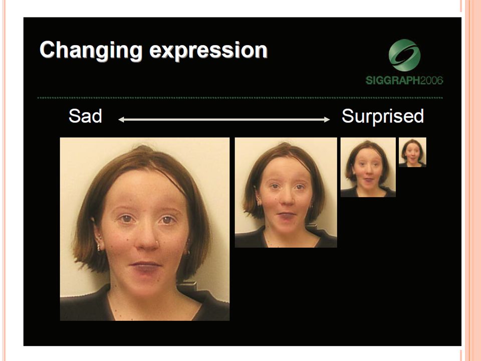
48. A PPLICATION : H YBRID I MAGES A. Oliva, A. Torralba, P.G. Schyns, “Hybrid Images,” SIGGRAPH 2006 “Hybrid Images,”

50. A PPLICATION : H YBRID I MAGES A. Oliva, A. Torralba, P.G. Schyns, “Hybrid Images,” SIGGRAPH 2006 “Hybrid Images,” Gaussian Filter Laplacian Filter

51. O UTLINE Image filter and convolution Convoluation and linear filter Gaussian filter, box filter, and median filter Application: Hybrid images Edge detection Image derivatives Gaussian derivative filters Canny edge detector

52. E DGE DETECTION Goal: Identify sudden changes (discontinuities) in an image Intuitively, most semantic and shape information from the image can be encoded in the edges More compact than pixels Ideal: artist’s line drawing (but artist is also using object-level knowledge) Source: D. Lowe

53. O RIGIN OF EDGES Edges are caused by a variety of factors: depth discontinuity surface color discontinuity illumination discontinuity surface normal discontinuity Source: Steve Seitz

54. C HARACTERIZING EDGES An edge is a place of rapid change in the image intensity function image intensity function (along horizontal scanline) first derivative edges correspond to extrema of derivative

55. O UTLINE Image filter and convolution Convoluation and linear filter Gaussian filter, box filter, and median filter Application: Hybrid images Edge detection Image derivatives Gaussian derivative filters Canny edge detector

56. D ERIVATIVES WITH CONVOLUTION For 2D function f(x,y), the partial derivative is: For discrete data, we can approximate using finite differences: To implement above as convolution, what would be the associated filter? Source: K. Grauman

57. P ARTIAL DERIVATIVES OF AN IMAGE Which shows changes with respect to x? -1 1 1 -1 or -1 1

58. F INITE DIFFERENCE FILTERS Other approximations of derivative filters exist: Source: K. Grauman

59. The gradient points in the direction of most rapid increase in intensity I MAGE GRADIENT The gradient of an image: The gradient direction is given by Source: Steve Seitz The edge strength is given by the gradient magnitude How does this direction relate to the direction of the edge?

60. O UTLINE Image filter and convolution Convolution and linear filter Gaussian filter, box filter, and median filter Application: Hybrid images Edge detection Image derivatives Gaussian derivative filters Canny edge detector

61. E FFECTS OF NOISE Consider a single row or column of the image Plotting intensity as a function of position gives a signal Where is the edge? Source: S. Seitz

62. S OLUTION : SMOOTH FIRST To find edges, look for peaks in f g f * g Source: S. Seitz

63. Differentiation is convolution, and convolution is associative: This saves us one operation: D ERIVATIVE THEOREM OF CONVOLUTION f Source: S. Seitz

64. D ERIVATIVE OF G AUSSIAN FILTER Are these filters separable? x-direction y-direction

65. D ERIVATIVE OF G AUSSIAN FILTER Which one finds horizontal/vertical edges? x-direction y-direction

66. Smoothed derivative removes noise, but blurs edge. Also finds edges at different “scales” 1 pixel3 pixels7 pixels S CALE OF G AUSSIAN DERIVATIVE FILTER Source: D. Forsyth

67. R EVIEW : S MOOTHING VS. DERIVATIVE FILTERS Smoothing filters Gaussian: remove “high-frequency” components; “low-pass” filter Can the values of a smoothing filter be negative? What should the values sum to? One: constant regions are not affected by the filter Derivative filters Derivatives of Gaussian Can the values of a derivative filter be negative? What should the values sum to? Zero: no response in constant regions High absolute value at points of high contrast

68. O UTLINE Image filter and convolution Convolution and linear filter Gaussian filter, box filter, and median filter Application: Hybrid images Edge detection Image derivatives Gaussian derivative filters Canny edge detector

69. T HE C ANNY EDGE DETECTOR original image The story of Lena Slide credit: Steve Seitz

70. T HE C ANNY EDGE DETECTOR norm of the gradient

71. T HE C ANNY EDGE DETECTOR thresholding

72. T HE C ANNY EDGE DETECTOR thresholding How to turn these thick regions of the gradient into curves?

73. N ON - MAXIMUM SUPPRESSION Check if pixel is local maximum along gradient direction, select single max across width of the edge requires checking interpolated pixels p and r

74. T HE C ANNY EDGE DETECTOR thinning (non-maximum suppression) Problem: pixels along this edge didn’t survive the thresholding

75. H YSTERESIS THRESHOLDING Use a high threshold to start edge curves, and a low threshold to continue them. Source: Steve Seitz

76. H YSTERESIS THRESHOLDING original image high threshold (strong edges) low threshold (weak edges) hysteresis threshold Source: L. Fei-Fei

77. R ECAP : C ANNY EDGE DETECTOR 1. Filter image with derivative of Gaussian 2. Find magnitude and orientation of gradient 3. Non-maximum suppression : Thin wide “ridges” down to single pixel width 4. Linking and thresholding ( hysteresis ): Define two thresholds: low and high Use the high threshold to start edge curves and the low threshold to continue them MATLAB: edge(image, ‘canny’); J. Canny, A Computational Approach To Edge Detection, IEEE Trans. Pattern Analysis and Machine Intelligence, 8:679-714, 1986.A Computational Approach To Edge Detection

78. E DGE DETECTION IS JUST THE BEGINNING … Berkeley segmentation database: http://www.eecs.berkeley.edu/Research/Projects/CS/vision/grouping/segbench/ http://www.eecs.berkeley.edu/Research/Projects/CS/vision/grouping/segbench/ image human segmentation gradient magnitude

79. BackgroundTexture Shadows Low-level edges vs. perceived contours Kristen Grauman, UT-Austin