Download presentation
Presentation is loading. Please wait.

1
Data Processing Dennis Shea National Center for Atmospheric Research NCAR is sponsored by the National Science Foundation

2
Data Processing Outline Coding principles Algebraic/logical expression operators Manual and automatic array creation if statements, do loops Built-in and Contributed functions User developed NCL functions/procedures User developed external procedures Sample processing Command Line Arguments [CLAs] Fortran external subroutines NCL as a scripting tool [time permitting] Global Variables [time permitting]
![Data Processing Outline Coding principles Algebraic/logical expression operators Manual and automatic array creation if statements, do loops Built-in and Contributed functions User developed NCL functions/procedures User developed external procedures Sample processing Command Line Arguments [CLAs] Fortran external subroutines NCL as a scripting tool [time permitting] Global Variables [time permitting]](http://images.slideplayer.com/35/10310523/slides/slide_2.jpg "Data Processing Outline Coding principles Algebraic/logical expression operators Manual and automatic array creation if statements, do loops Built-in and Contributed functions User developed NCL functions/procedures User developed external procedures Sample processing Command Line Arguments [CLAs] Fortran external subroutines NCL as a scripting tool [time permitting] Global Variables [time permitting]")
3
1. Clear and simple code is best 2. Indent code blocks 3. Use descriptive variable names 4. Comment code segments and overall objectives 5. Use built-in functions: efficiency 6. Create functions to perform repetitive tasks 7. Use parameters in place of hard-coded numbers 8. Test code segments (unit testing) Data Processing: Coding
 Data Processing: Coding.")
4
Logical Relational (Boolean) Operators Same as fortran-77.le.less than or equal.lt.less than.ge.greater than or equal to.gt.greater than.ne.not equal.eq.equal.and.and.not.not.or.or.and..not..or. combine logical expressions

5
Algebraic Operators All support scalar and array operations -Subtraction / Negation +Addition / String concatenation *Multiplication /Divide %Modulus (integers only) >Greater than selection <Less-than selection #Matrix multiply ^Exponentiation
 >Greater than selection <Less-than selection #Matrix multiply ^Exponentiation")
6
algebraic operator and string concatenator: x = “alpha_” + (5.3 + 7) + “_beta” x = “alpha_12.3_beta” Algebraic Operators algebraic operator: x = 5.3 + 7.95 x = 13.25 concatenate string: str = “pine” + “apple” str = “pineapple” + is an overloaded operator (…) allows you to circumvent precedence rules
 + _beta x = alpha_12.3_beta Algebraic Operators algebraic operator: x = x = concatenate string: str = pine + apple str = pineapple + is an overloaded operator (…) allows you to circumvent precedence rules")
7
Manual Array Creation (1) array constructor characters (/…/) – a_integer= (/1, 9, -4/) – a_float = (/1.0, -2e3, 3.0/) – a_double = (/1, 2.0, 3.2d /) – a_string = (/"abc",”12345",”hello world"/) – a_logical = (/True, False, True/) – a_2darray= (/ (/1,2,3/), (/4,5,6/), (/7,8,9/) /)
 array constructor characters (/…/) – a_integer= (/1, 9, -4/) – a_float = (/1.0, -2e3, 3.0/) – a_double = (/1, 2.0, 3.2d /) – a_string = (/ abc , , hello world /) – a_logical = (/True, False, True/) – a_2darray= (/ (/1,2,3/), (/4,5,6/), (/7,8,9/) /)")
8
Manual Array Creation (2) new function [Fortran dimension, allocate ; C malloc] – x = new (array_size/shape, type, _FillValue) – _FillValue is optional [assigned default if not specified] – “No_FillValue” means no missing value assigned – a = new(3, float) – b = new(10, double, 1d20) – c = new( (/5, 6, 7/), integer) – d = new(dimsizes(U), string) – e = new(dimsizes(ndtooned(U)), logical) new and (/…/) can appear anywhere in script – new is not used that often
![Manual Array Creation (2) new function [Fortran dimension, allocate ; C malloc] – x = new (array_size/shape, type, _FillValue) – _FillValue is optional [assigned default if not specified] – No_FillValue means no missing value assigned – a = new(3, float) – b = new(10, double, 1d20) – c = new( (/5, 6, 7/), integer) – d = new(dimsizes(U), string) – e = new(dimsizes(ndtooned(U)), logical) new and (/…/) can appear anywhere in script – new is not used that often](http://images.slideplayer.com/35/10310523/slides/slide_8.jpg "Manual Array Creation (2) new function [Fortran dimension, allocate ; C malloc] – x = new (array_size/shape, type, _FillValue) – _FillValue is optional [assigned default if not specified] – No_FillValue means no missing value assigned – a = new(3, float) – b = new(10, double, 1d20) – c = new( (/5, 6, 7/), integer) – d = new(dimsizes(U), string) – e = new(dimsizes(ndtooned(U)), logical) new and (/…/) can appear anywhere in script – new is not used that often")
9
Automatic Array Creation variable to variable assignment – y = x y => same size, type as x plus meta data – no need to pre-allocate space for y data importation via supported format – u = f->U ; all associated meta data – same for subset of data: u = f->U(:, 3:9:2, :, 10:20) – meta data (coordinate array will reflect subset) functions – return array: no need to pre-allocate space – grido = f2fsh ( gridi, (/ 73,144 /)) – gridi(10,30,181,360) grido(10,30,73,144)
 – meta data (coordinate array will reflect subset) functions – return array: no need to pre-allocate space – grido = f2fsh ( gridi, (/ 73,144 /)) – gridi(10,30,181,360) grido(10,30,73,144)")
10
Array Dimension Rank Reduction singleton dimensions eliminated (subtle point) let T(12,64,128) – Tjan = T(0, :, :) Tjan(64,128) – Tjan automatically becomes 2D: Tjan(64,128) – array rank reduced; ‘degenerate’ dimension – all applicable meta data copied can override dimension rank reduction – Tjan = T(0:0, :, :) Tjan(1,64,128) – TJAN = new( (/1,64,128/), typeof(T), T@_FillValue) TJAN(0,:,:) = T(0,:,:) Dimension Reduction is a "feature" [really ]
![Array Dimension Rank Reduction singleton dimensions eliminated (subtle point) let T(12,64,128) – Tjan = T(0, :, :) Tjan(64,128) – Tjan automatically becomes 2D: Tjan(64,128) – array rank reduced; ‘degenerate’ dimension – all applicable meta data copied can override dimension rank reduction – Tjan = T(0:0, :, :) Tjan(1,64,128) – TJAN = new( (/1,64,128/), typeof(T), TJAN(0,:,:) = T(0,:,:) Dimension Reduction is a feature [really ]](http://images.slideplayer.com/35/10310523/slides/slide_10.jpg "Array Dimension Rank Reduction singleton dimensions eliminated (subtle point) let T(12,64,128) – Tjan = T(0, :, :) Tjan(64,128) – Tjan automatically becomes 2D: Tjan(64,128) – array rank reduced; ‘degenerate’ dimension – all applicable meta data copied can override dimension rank reduction – Tjan = T(0:0, :, :) Tjan(1,64,128) – TJAN = new( (/1,64,128/), typeof(T), TJAN(0,:,:) = T(0,:,:) Dimension Reduction is a feature [really ]")
11
Array Syntax/Operators Similar to array languages like: f90/f95, Matlab, IDL Arrays must conform: same size and shape Scalars automatically conform to all array sizes Non-conforming arrays: use built-in conform function All array operations automatically ignore _FillValue Use of array syntax is essential for efficiency

12
Array Syntax/Operators arrays must be same size and shape: conform let A and B be (10,30,64,128) <= conform – C = A+B <= C(10,30,64,128) – D = A-B – E = A*B – C, D, E created if they did not previously exist
 <= conform – C = A+B <= C(10,30,64,128) – D = A-B – E = A*B – C, D, E created if they did not previously exist")
13
Array Syntax/Operators (2) let T and P be (10,30,180,360) ; conforming arrays – theta = T*(1000/P)^0.286 theta(10,30,180,360) non-conforming arrays; use built-in conform function – Let T be (30,30,64,128) and P be (30) then – theta = T*(1000/conform(T,P,1))^0.286 let SST be (100,72,144) and SICE = -1.8 (scalar) – SST = SST > SICE [f90: where (sst.lt.sice) sst = sice] – operation performed by is called clipping all array operations automatically ignore _FillValue
![Array Syntax/Operators (2) let T and P be (10,30,180,360) ; conforming arrays – theta = T*(1000/P)^0.286 theta(10,30,180,360) non-conforming arrays; use built-in conform function – Let T be (30,30,64,128) and P be (30) then – theta = T*(1000/conform(T,P,1))^0.286 let SST be (100,72,144) and SICE = -1.8 (scalar) – SST = SST > SICE [f90: where (sst.lt.sice) sst = sice] – operation performed by is called clipping all array operations automatically ignore _FillValue](http://images.slideplayer.com/35/10310523/slides/slide_13.jpg "Array Syntax/Operators (2) let T and P be (10,30,180,360) ; conforming arrays – theta = T*(1000/P)^0.286 theta(10,30,180,360) non-conforming arrays; use built-in conform function – Let T be (30,30,64,128) and P be (30) then – theta = T*(1000/conform(T,P,1))^0.286 let SST be (100,72,144) and SICE = -1.8 (scalar) – SST = SST > SICE [f90: where (sst.lt.sice) sst = sice] – operation performed by is called clipping all array operations automatically ignore _FillValue")
14
Conditional/Repetitive Execution if : conditional execution of one or more statements do : loops; fixed repetitions; for other languages do while : until some condition is met where : conditional/repetitive execution

15
if blocks (1) if-then-end if ; note: end if has space if ( all(a.gt.0.) ) then ; then is optional …statements end if ; space is required if-then-else-end if if ( any(ismissing(a)) ) then …statements else …statements end if lazy expression evaluation [left-to-right] if ( any(b.lt.0.).and. all(a.gt.0.) ) then …statements end if
![if blocks (1) if-then-end if ; note: end if has space if ( all(a.gt.0.) ) then ; then is optional …statements end if ; space is required if-then-else-end if if ( any(ismissing(a)) ) then …statements else …statements end if lazy expression evaluation [left-to-right] if ( any(b.lt.0.).and.](http://images.slideplayer.com/35/10310523/slides/slide_15.jpg "all(a.gt.0.) ) then …statements end if.")
16
if blocks (2) Technically, no ‘else if’ block but if blocks can be nested str = "MAR” if (str.eq."JAN") then print("January") else if (str.eq."FEB") then print("February") else if (str.eq."MAR") then print("March") else if (str.eq."APR") then print("April") else print("Enough of this!") end if ; must group all ‘end if’ end if ; at the end end if ; not very clear end if
 Technically, no ‘else if’ block but if blocks can be nested str = MAR if (str.eq. JAN ) then print( January ) else if (str.eq. FEB ) then print( February ) else if (str.eq. MAR ) then print( March ) else if (str.eq. APR ) then print( April ) else print( Enough of this! ) end if ; must group all ‘end if’ end if ; at the end end if ; not very clear end if")
17
do loops (1) do : code segments repeatedly executed ‘n’ times Use of multiple embedded do loops should be minimized + Generally true with any interpreted language See if array syntax can be used Use fortran or C for deep embedded do loops
 do : code segments repeatedly executed ‘n’ times Use of multiple embedded do loops should be minimized + Generally true with any interpreted language See if array syntax can be used Use fortran or C for deep embedded do loops")
18
do loops (2) do n=nStrt, nLast [,stride] ; all scalars; stride always positive...statements... end do do n=nLast, nStrt, 5 ; nLast>nStrt decreases each iteration...statements... end do do-end do (note: end do has space) do i=scalar_start_exp, scalar_end_exp [, scalar_stride_exp]...statements... end do stride always positive; default is one (1)
![do loops (2) do n=nStrt, nLast [,stride] ; all scalars; stride always positive...statements...](http://images.slideplayer.com/35/10310523/slides/slide_18.jpg "end do do n=nLast, nStrt, 5 ; nLast>nStrt decreases each iteration...statements... end do do-end do (note: end do has space) do i=scalar_start_exp, scalar_end_exp [, scalar_stride_exp]...statements... end do stride always positive; default is one (1).")
19
do loops (3) Sequential loop execution my be altered break: based on some condition exit current loop do i=iStrt, iLast...statements... if (foo.gt 1000) then dum = 3*sqrt(foo) ; optional...statements... break ; go to statement after end do end if...statements... end do...statements... ; first statement after end do
 then dum = 3*sqrt(foo) ; optional...statements... break ; go to statement after end do end if...statements... end do...statements... ; first statement after end do.")
20
do loops (4) Sequential loop execution my be altered continue: based on some condition go to next iteration do i=iStrt, iLast...statements... if (foo.gt 1000) then continue ; go to end do and next iteration end if...statements... end do
 then continue ; go to end do and next iteration end if...statements... end do.")
21
do while undefined number of iterations do while: based on some condition, exit loop do while (foo.gt.1000)...statements... foo = ; will go to 1st statement after end do ; when ‘foo’ > 1000...statements... end do...statements...

22
do: Tips and Errors NCL array subscripting (indexing) starts at 0 not 1. Let x(ntim,…) do nt=0,ntim-1 NOT => do nt=1,ntim foo = func(x(nt,…)..) end do Use := syntax when arrays may change size within a loop do yyyy=nyrStrt, nyrLast ; loop over daily files (leap years+1 file) fili := systemfunc(“ls 3B42_daily.”+yyyy+”.nc”) ; (365 or 366) q := addfiles(fili, “r”) p := q[:]->rain ; (365 or 366, nlat,mlon) end do Else. if you had used the standard assignment = you would get the dreaded fatal:Dimension sizes of left hand side and right hand side of assignment do not match Prior to v6.1.1, variables had to be explicitly deleted delete( [/ fili, q, p /] )
 do nt=0,ntim-1 NOT => do nt=1,ntim foo = func(x(nt,…)..) end do Use := syntax when arrays may change size within a loop do yyyy=nyrStrt, nyrLast ; loop over daily files (leap years+1 file) fili := systemfunc( ls 3B42_daily. +yyyy+ .nc ) ; (365 or 366) q := addfiles(fili, r ) p := q[:]->rain ; (365 or 366, nlat,mlon) end do Else. if you had used the standard assignment = you would get the dreaded fatal:Dimension sizes of left hand side and right hand side of assignment do not match Prior to v6.1.1, variables had to be explicitly deleted delete( [/ fili, q, p /] ).")
23
Built-in Functions and Procedures NCL continually adds I/O, Graphics, Functions Objective: meet evolving community needs internal (CGD, WRF, …) ncl-talk workshops
 ncl-talk workshops")
24
Built-in Functions and Procedures use whenever possible learn and use utility functions (any language) – all, any, conform, ind, ind_resolve, dimsizes, num – fspan, ispan, ndtooned, onedtond, reshape – mask, ismissing, str* – system, systemfunc – cd_calendar, cd_inv_calendar – to* (toint, tofloat, …); round, short2flt, …. – where – sort, sqsort, dim_pqsort_n, dim_sort_n – generate_sample_indices (6.3.0) [bootstrap] – get_cpu_time, wallClockElapseTime
 [bootstrap] – get_cpu_time, wallClockElapseTime.")
25
Built-in Functions and Procedures common computational functions – dim_*_n, where – avg, stddev, min, max, …. – escorc, pattern_cor, esccr, esacr (correlation) – rtest, ttest, ftest, kolsm2_n – regression/trend: regline_stats, trend_manken_n (6.3.0) – filtering: filwgts_lanczos, dim_bfband_n (6.3.0) – eofunc, eofunc_ts, eof_varimax – diagnostics: MJO, Space-Time, POP, kmeans (6.3.0) – regridding: linint2, ESMF, … – random number generators – climatology & anomaly (hrly, daily, monthly,…) – wgt_areaave, wgt_arearmse,… – fft: ezfftf, ezfftb, fft2d, specx_anal, specxy_anal – spherical harmonic: synthesis, analysis, div, vort, regrid
 – rtest, ttest, ftest, kolsm2_n – regression/trend: regline_stats, trend_manken_n (6.3.0) – filtering: filwgts_lanczos, dim_bfband_n (6.3.0) – eofunc, eofunc_ts, eof_varimax – diagnostics: MJO, Space-Time, POP, kmeans (6.3.0) – regridding: linint2, ESMF, … – random number generators – climatology & anomaly (hrly, daily, monthly,…) – wgt_areaave, wgt_arearmse,… – fft: ezfftf, ezfftb, fft2d, specx_anal, specxy_anal – spherical harmonic: synthesis, analysis, div, vort, regrid.")
26
dimsizes(x) returns the dimension sizes of a variable will return 1D array of integers if the array queried is multi-dimensional. fin = addfile(“in.nc”,”r”) t = fin->T dimt = dimsizes(t) print(dimt) rank = dimsizes(dimt) print ("rank="+rank) Variable: dimt Type: integer Total Size: 16 bytes 4 values Number of dimensions: 1 Dimensions and sizes:(4) (0) 12 (1) 25 (2) 116 (3) 100 (0) rank=4
 t = fin->T dimt = dimsizes(t) print(dimt) rank = dimsizes(dimt) print ( rank= +rank) Variable: dimt Type: integer Total Size: 16 bytes 4 values Number of dimensions: 1 Dimensions and sizes:(4) (0) 12 (1) 25 (2) 116 (3) 100 (0) rank=4.")
27
ispan( start:integer, finish:integer, stride:integer ) returns a 1D array of integers – beginning with start and ending with finish. time = ispan(1990,2001,2) print(time) Variable: time Type: integer Number of Dimensions: 1 Dimensions and sizes:(6) (0) 1990 (1) 1992 (2) 1994 (3) 1996 (4) 1998 (5) 2000
 print(time) Variable: time Type: integer Number of Dimensions: 1 Dimensions and sizes:(6) (0) 1990 (1) 1992 (2) 1994 (3) 1996 (4) 1998 (5)")
28
ispan, sprinti People want ‘zero filled’ two digit field month = (/ ”01”,”02”, ”03”,”04”, ”05”,”06” \, ”07”,”08”, ”09”,”10”, ”11”,”12” /) day = (/ ”01”,”02”, ”03”,”04”, ”05”,”06” \, ”07”,”08”, ”09”,”10”, ”11”,”12” \, ….., “30”,”31”) cleaner / nicer code: month = sprinti("%0.2i", ispan(1,12,1) ) day = sprinti("%0.2i", ispan(1,31,1) ) year = “” + ispan(1900,2014,1)
 day = (/ 01 , 02 , 03 , 04 , 05 , 06 \, 07 , 08 , 09 , 10 , 11 , 12 \, ….., 30 , 31 ) cleaner / nicer code: month = sprinti( %0.2i , ispan(1,12,1) ) day = sprinti( %0.2i , ispan(1,31,1) ) year = + ispan(1900,2014,1)")
29
fspan( start:numeric, finish:numeric, n:integer ) b = fsp an( -89.125, 9.3, 100) print(b) Variable b: Type: float Number of Dimensions: 1 Dimensions and sizes:(100) (0) -89.125 (1) -88.13081 (2) -87.13662 (…) …. (97) 7.311615 (98) 8.305809 (99) 9.3 1D array of evenly spaced float/double values npts is the integer number of points including start and finish values d = fsp an( -89.125, 9.3d0, 100) print(d) ; type double
 (98) (99) 9.3 1D array of evenly spaced float/double values npts is the integer number of points including start and finish values d = fsp an( , 9.3d0, 100) print(d) ; type double.")
30
ismissing, num, all, any,.not. if (any( ismissing(xOrig) )) then …. else …. end if ismissing MUST be used to check for _FillValue attribute if ( x.eq. x@_FillValue ) will NOT work x = (/ 1,2, -99, 4, -99, -99, 7 /) ; x@_FillValue = -99 xmsg = ismissing(x) => (/ False, False, True, False, True, True, False /) often used in combination with array functions if (all( ismissing(x) )) then … [else …] end if nFill = num( ismissing(x) ) nVal = num(.not. ismissing(x) )
 will NOT work x = (/ 1,2, -99, 4, -99, -99, 7 /) ; = -99 xmsg = ismissing(x) => (/ False, False, True, False, True, True, False /) often used in combination with array functions if (all( ismissing(x) )) then … [else …] end if nFill = num( ismissing(x) ) nVal = num(.not. ismissing(x) ).")
31
mask sets values to _FillValue that DO NOT equal mask array in = addfile(“atmos.nc","r") ts = in->TS(0,:,:) oro = in->ORO(0,:,:) ; mask ocean ; [ocean=0, land=1, sea_ice=2] ts = mask(ts,oro,1) NCL has 1 degree land-sea mask available [landsea_mask] – load "$NCARG_ROOT/lib/ncarg/nclscripts/csm/shea_util.ncl” – flags for ocean, land, lake, small island, ice shelf
![mask sets values to _FillValue that DO NOT equal mask array in = addfile( atmos.nc , r ) ts = in->TS(0,:,:) oro = in->ORO(0,:,:) ; mask ocean ; [ocean=0, land=1, sea_ice=2] ts = mask(ts,oro,1) NCL has 1 degree land-sea mask available [landsea_mask] – load $NCARG_ROOT/lib/ncarg/nclscripts/csm/shea_util.ncl – flags for ocean, land, lake, small island, ice shelf](http://images.slideplayer.com/35/10310523/slides/slide_31.jpg "mask sets values to _FillValue that DO NOT equal mask array in = addfile( atmos.nc , r ) ts = in->TS(0,:,:) oro = in->ORO(0,:,:) ; mask ocean ; [ocean=0, land=1, sea_ice=2] ts = mask(ts,oro,1) NCL has 1 degree land-sea mask available [landsea_mask] – load $NCARG_ROOT/lib/ncarg/nclscripts/csm/shea_util.ncl – flags for ocean, land, lake, small island, ice shelf")
32
where ; q is an array; q q=q+256 ; f90: where(q.lt.0) q=q+256 ; NCL: q = where (q.lt.0, q+256, q) performs array assignments based upon a conditional array function where(conditional_expression \, true_value(s) \, false_value(s) ) similar to f90 “where” statement components evaluated separately via array operations x = where (T.ge.0.and. ismissing(Z), a+25, 1.8*b) salinity = where (sst.lt.5.and. ice.gt.icemax \, salinity*0.9, salinity) can not do: y = where(y.eq.0, y@_FillValue, 1./y) instead use: y = 1.0/where(y.eq.0, y@_FillValue, y)
, a+25, 1.8*b) salinity = where (sst.lt.5.and. ice.gt.icemax \, salinity*0.9, salinity) can not do: y = where(y.eq.0, 1./y) instead use: y = 1.0/where(y.eq.0, y).")
33
dim_*_n [dim_*] perform common operations on an array dimension(s) - dim_avg_n (stddev, sum, sort, median, rmsd,…) dim_*_n functions operate on a user specified dimension - use less memory, cleaner code than older dim_* dim_* functions are original (old) interfaces; deprecated - operate on rightmost dimension only - may require dimension reordering - kept for backward compatibility Recommendation: use dim_*_n
![dim_*_n [dim_*] perform common operations on an array dimension(s) - dim_avg_n (stddev, sum, sort, median, rmsd,…) dim_*_n functions operate on a user specified dimension - use less memory, cleaner code than older dim_* dim_* functions are original (old) interfaces; deprecated - operate on rightmost dimension only - may require dimension reordering - kept for backward compatibility Recommendation: use dim_*_n](http://images.slideplayer.com/35/10310523/slides/slide_33.jpg "dim_*_n [dim_*] perform common operations on an array dimension(s) - dim_avg_n (stddev, sum, sort, median, rmsd,…) dim_*_n functions operate on a user specified dimension - use less memory, cleaner code than older dim_* dim_* functions are original (old) interfaces; deprecated - operate on rightmost dimension only - may require dimension reordering - kept for backward compatibility Recommendation: use dim_*_n")
34
dim_*_n [dim_*] dim_avg_n: Consider: x(ntim,nlat,mlon) => x(0,1,2) function dim_avg_n( x, n ) => operate on dim n xZon = dim_avg_n( x, 2 ) => xZon(ntim,nlat) xTim = dim_avg_n( x, 0 ) => xTim(nlat,mlon) dim_avg: Consider: x(ntim,nlat,mlon) function dim_avg ( x ) => operate on rightmost dim xZon = dim_avg( x ) => xZon(ntim,nlat) xTim = dim_avg( x(lat|:,lon|:,time|:) ) => xTim(nlat,mlon)
![dim_*_n [dim_*] dim_avg_n: Consider: x(ntim,nlat,mlon) => x(0,1,2) function dim_avg_n( x, n ) => operate on dim n xZon = dim_avg_n( x, 2 ) => xZon(ntim,nlat) xTim = dim_avg_n( x, 0 ) => xTim(nlat,mlon) dim_avg: Consider: x(ntim,nlat,mlon) function dim_avg ( x ) => operate on rightmost dim xZon = dim_avg( x ) => xZon(ntim,nlat) xTim = dim_avg( x(lat|:,lon|:,time|:) ) => xTim(nlat,mlon)](http://images.slideplayer.com/35/10310523/slides/slide_34.jpg "dim_*_n [dim_*] dim_avg_n: Consider: x(ntim,nlat,mlon) => x(0,1,2) function dim_avg_n( x, n ) => operate on dim n xZon = dim_avg_n( x, 2 ) => xZon(ntim,nlat) xTim = dim_avg_n( x, 0 ) => xTim(nlat,mlon) dim_avg: Consider: x(ntim,nlat,mlon) function dim_avg ( x ) => operate on rightmost dim xZon = dim_avg( x ) => xZon(ntim,nlat) xTim = dim_avg( x(lat|:,lon|:,time|:) ) => xTim(nlat,mlon)")
35
conform, conform_dims function conform( x, r, ndim ) function conform_dims( dims, r, ndim ) Array operations require that arrays conform array r is ‘broadcast’ (replicated) to array sizes of x expand array (r) to match (x) on dimensions sizes (dims) ndim: scalar or array (integer) indicating which dimension(s) of x or dims match the dimensions of array x(nlat,mlon), w(nlat) ; x( 0, 1), w( 0 ) wx = conform (x, w, 0) ; wx(nlat,mlon) xwx = x*wx ; xwx = x* conform (x, w, 0) xar = sum(xwx)/sum(wx) ; area avg (wgt_areaave,…)
 function conform_dims( dims, r, ndim ) Array operations require that arrays conform array r is ‘broadcast’ (replicated) to array sizes of x expand array (r) to match (x) on dimensions sizes (dims) ndim: scalar or array (integer) indicating which dimension(s) of x or dims match the dimensions of array x(nlat,mlon), w(nlat) ; x( 0, 1), w( 0 ) wx = conform (x, w, 0) ; wx(nlat,mlon) xwx = x*wx ; xwx = x* conform (x, w, 0) xar = sum(xwx)/sum(wx) ; area avg (wgt_areaave,…)")
36
conform, conform_dims T(ntim, klev, nlat,mlon), dp(klev) ( 0, 1, 2, 3 ) dpT = conform (T, dp, 1) ; dpT(ntim,klev,nlat,mlon) T_wgtAve = dim_sum_n (T*dpT, 1)/dim_sum_n(dp, 0) ; T_wgtAve(ntim,nlat,mlon) Let T(30,30,64,128), P be (30). ( 0, 1, 2, 3 ) <= dimension numbers theta = T*(1000/conform(T,P,1))^0.286 ; theta(30,30,64,128)
 <= dimension numbers theta = T*(1000/conform(T,P,1))^0.286 ; theta(30,30,64,128).")
37
conform, conform_dims function pot_temp_n (p:numeric, t:numeric, ndim[*]:integer, opt:integer) ; Compute potential temperature; any dimensionality begin rankp = dimsizes(dimsizes(p)) rankt = dimsizes(dimsizes(t)) p0 = 100000. ; default [units = Pa] if (rankp.eq.rankt) then theta = t*(p0/p)^0.286 ; conforming arrays else theta = t*(p0/conform(t,p,ndim))^0.286 ; non-conforming end if theta@long_name = "potential temperature” ; meta data theta@units = "K” copy_VarCoords (t, theta) ; copy coordinates return( theta ) end
![conform, conform_dims function pot_temp_n (p:numeric, t:numeric, ndim[*]:integer, opt:integer) ; Compute potential temperature; any dimensionality begin rankp = dimsizes(dimsizes(p)) rankt = dimsizes(dimsizes(t)) p0 =](http://images.slideplayer.com/35/10310523/slides/slide_37.jpg "; default [units = Pa] if (rankp.eq.rankt) then theta = t*(p0/p)^0.286 ; conforming arrays else theta = t*(p0/conform(t,p,ndim))^0.286 ; non-conforming end if = potential temperature ; meta data = K copy_VarCoords (t, theta) ; copy coordinates return( theta ) end.")
38
ind ; let x(:), y(:), z(:) [z@_FillValue] ; create triplet with only ‘good’ values iGood = ind (.not. ismissing(z) ) xGood = x(iGood) yGood = y(iGood) zGood = z(iGood) ind operates on 1D array only – returns indices of elements that evaluate to True – generically similar to IDL “where” and Matlab “find” [returns indices] ; let a(:), return subscripts can be on lhs ii = ind (a.gt.500 ) a(ii) = 3*a(ii) +2 Should check the returned subscript to see if it is missing – if (any(ismissing(ii))) then …. end if
 ) xGood = x(iGood) yGood = y(iGood) zGood = z(iGood) ind operates on 1D array only – returns indices of elements that evaluate to True – generically similar to IDL where and Matlab find [returns indices] ; let a(:), return subscripts can be on lhs ii = ind (a.gt.500 ) a(ii) = 3*a(ii) +2 Should check the returned subscript to see if it is missing – if (any(ismissing(ii))) then …. end if.")
39
ind, ndtooned, onedtond ; let q and x be nD arrays q1D = ndtooned (q) x1D = ndtooned (x) ii = ind(q1D.gt.0..and. q1D.lt.5) jj = ind(q1D.gt.25) kk = ind(q1D.lt. -50) x1D(ii) = sqrt( q1D(ii) ) x1D(jj) = 72 x1D(kk) = -x1D(kk)*3.14159 x = onedtond(x1D, dimsizes(x)) ind operates on 1D array only – if nD … use with ndtooned; reconstruct with onedtond, dimsizes
 jj = ind(q1D.gt.25) kk = ind(q1D.lt. -50) x1D(ii) = sqrt( q1D(ii) ) x1D(jj) = 72 x1D(kk) = -x1D(kk)* x = onedtond(x1D, dimsizes(x)) ind operates on 1D array only – if nD … use with ndtooned; reconstruct with onedtond, dimsizes.")
40
User function: ind, ndtooned, onedtond function change_x(q:numeric, x:numeric) begin q1D = ndtooned (q) x1D = ndtooned (x) ii = ind(q1D.gt.0..and. q1D.lt.5) jj = ind(q1D.gt.25) kk = ind(q1D.lt. -50) x1D(ii) = sqrt( q1D(ii) ) x1D(jj) = 72 x1D(kk) = -x1D(kk)*3.14159 x = onedtond(x1D, dimsizes(x)) x@info = “x after changes based on q” return(x) end
 jj = ind(q1D.gt.25) kk = ind(q1D.lt. -50) x1D(ii) = sqrt( q1D(ii) ) x1D(jj) = 72 x1D(kk) = -x1D(kk)* x = onedtond(x1D, dimsizes(x)) = x after changes based on q return(x) end.")
41
date: cd_calendar, cd_inv_calendar Date/time functions: – http://www.ncl.ucar.edu/Document/Functions/date.shtml http://www.ncl.ucar.edu/Document/Functions/date.shtml – cd_calendar, cd_inv_calendar time = (/ 17522904, 17522928, 17522952/) time@units = “hours since 1-1-1 00:00:0.0” date = cd_calendar(time, 0) print(date) Variable: date Type: float Total Size: 72 bytes 18 values Number of Dimensions: 2 Dimensions and sizes: [3] x [6] (0,0:5) 2000 1 1 0 0 0 (1,0:5) 2000 1 2 0 0 0 (2,0:5) 2000 1 3 0 0 0 TIME = cd_inv_calendar (iyr, imo, iday, ihr, imin, sec \,“hours since 1-1-1 00:00:0.0”,0) date = cd_calendar(time,-2) print(date) Variable: date Type: integer Total Size: 12 bytes 3 values Number of Dimensions: 1 Dimensions and sizes: [3] (0) 20000101 (1) 20000102 (2) 20000103
![date: cd_calendar, cd_inv_calendar Date/time functions: – – cd_calendar, cd_inv_calendar time = (/ , , /) = hours since :00:0.0 date = cd_calendar(time, 0) print(date) Variable: date Type: float Total Size: 72 bytes 18 values Number of Dimensions: 2 Dimensions and sizes: [3] x [6] (0,0:5) (1,0:5) (2,0:5) TIME = cd_inv_calendar (iyr, imo, iday, ihr, imin, sec \, hours since :00:0.0 ,0) date = cd_calendar(time,-2) print(date) Variable: date Type: integer Total Size: 12 bytes 3 values Number of Dimensions: 1 Dimensions and sizes: [3] (0) (1) (2)](http://images.slideplayer.com/35/10310523/slides/slide_41.jpg "date: cd_calendar, cd_inv_calendar Date/time functions: – – cd_calendar, cd_inv_calendar time = (/ , , /) = hours since :00:0.0 date = cd_calendar(time, 0) print(date) Variable: date Type: float Total Size: 72 bytes 18 values Number of Dimensions: 2 Dimensions and sizes: [3] x [6] (0,0:5) (1,0:5) (2,0:5) TIME = cd_inv_calendar (iyr, imo, iday, ihr, imin, sec \, hours since :00:0.0 ,0) date = cd_calendar(time,-2) print(date) Variable: date Type: integer Total Size: 12 bytes 3 values Number of Dimensions: 1 Dimensions and sizes: [3] (0) (1) (2)")
42
cd_calendar, ind f = addfile("...", "r) ; f = addfiles(fils, "r”) ; ALL times on file TIME = f->time ; TIME = f[:]->time YYYYMM = cd_calendar(TIME, -1) ; convert ymStrt = 190801 ; year-month start ymLast = 200712 ; year-month last iStrt = ind(YYYYMM.eq.ymStrt) ; index of start time iLast = ind(YYYYMM.eq.ymLasrt) ; last time x = f->X(iStrt:iLast,...) ; read only specified time period xAvg = dim_avg_n (x, 0) ; dim_avg_n_Wrap ;===== specify and read selected dates; compositing ymSelect = (/187703, 190512, 194307,..., 201107 /) iSelect = get1Dindex(TIME, ymSelect) ; contributed.ncl xSelect = f->X(iSelect,...) ; read selected times only xSelectAvg = = dim_avg_n (xSelect, 0) ; dim_avg_n_Wrap
![cd_calendar, ind f = addfile( ... , r) ; f = addfiles(fils, r ) ; ALL times on file TIME = f->time ; TIME = f[:]->time YYYYMM = cd_calendar(TIME, -1) ; convert ymStrt = ; year-month start ymLast = ; year-month last iStrt = ind(YYYYMM.eq.ymStrt) ; index of start time iLast = ind(YYYYMM.eq.ymLasrt) ; last time x = f->X(iStrt:iLast,...) ; read only specified time period xAvg = dim_avg_n (x, 0) ; dim_avg_n_Wrap ;===== specify and read selected dates; compositing ymSelect = (/187703, , ,..., /) iSelect = get1Dindex(TIME, ymSelect) ; contributed.ncl xSelect = f->X(iSelect,...) ; read selected times only xSelectAvg = = dim_avg_n (xSelect, 0) ; dim_avg_n_Wrap](http://images.slideplayer.com/35/10310523/slides/slide_42.jpg "cd_calendar, ind f = addfile( ... , r) ; f = addfiles(fils, r ) ; ALL times on file TIME = f->time ; TIME = f[:]->time YYYYMM = cd_calendar(TIME, -1) ; convert ymStrt = ; year-month start ymLast = ; year-month last iStrt = ind(YYYYMM.eq.ymStrt) ; index of start time iLast = ind(YYYYMM.eq.ymLasrt) ; last time x = f->X(iStrt:iLast,...) ; read only specified time period xAvg = dim_avg_n (x, 0) ; dim_avg_n_Wrap ;===== specify and read selected dates; compositing ymSelect = (/187703, , ,..., /) iSelect = get1Dindex(TIME, ymSelect) ; contributed.ncl xSelect = f->X(iSelect,...) ; read selected times only xSelectAvg = = dim_avg_n (xSelect, 0) ; dim_avg_n_Wrap")
43
str_* [string functions] x = (/ “u_052134_C”, “q_1234_C”, “temp_72.55_C”/) var_x = str_get_field( x, 1, “_”) result: var_x = (/”u”, “q”, “temp”/) ; strings ; -------- col_x = str_get_cols( x, 2, 4) result: col_x = (/”052”, “123”, “mp_” /) ; strings ;--------- N = toint( str_get_cols( x(0), 3, 7) ) ; N=52134 (integer) T = tofloat( str_get_cols( x(2), 5,9 ) ) ; T=72.55 (float) many new str_* functions http://www.ncl.ucar.edu/Document/Functions/string.shtml greatly enhance ability to handle strings can be used to unpack ‘complicated’ string arrays
![str_* [string functions] x = (/ u_052134_C , q_1234_C , temp_72.55_C /) var_x = str_get_field( x, 1, _ ) result: var_x = (/ u , q , temp /) ; strings ; col_x = str_get_cols( x, 2, 4) result: col_x = (/ 052 , 123 , mp_ /) ; strings ; N = toint( str_get_cols( x(0), 3, 7) ) ; N=52134 (integer) T = tofloat( str_get_cols( x(2), 5,9 ) ) ; T=72.55 (float) many new str_* functions greatly enhance ability to handle strings can be used to unpack ‘complicated’ string arrays](http://images.slideplayer.com/35/10310523/slides/slide_43.jpg "str_* [string functions] x = (/ u_052134_C , q_1234_C , temp_72.55_C /) var_x = str_get_field( x, 1, _ ) result: var_x = (/ u , q , temp /) ; strings ; col_x = str_get_cols( x, 2, 4) result: col_x = (/ 052 , 123 , mp_ /) ; strings ; N = toint( str_get_cols( x(0), 3, 7) ) ; N=52134 (integer) T = tofloat( str_get_cols( x(2), 5,9 ) ) ; T=72.55 (float) many new str_* functions greatly enhance ability to handle strings can be used to unpack ‘complicated’ string arrays")
44
system, systemfunc (1 of 2) system passes to the shell a command to perform an action NCL executes the Bourne shell (can be changed) create a directory if it does not exist (Bourne shell syntax) DIR = “/ptmp/shea/SAMPLE” system (“if ! test –d “+DIR+” ; then mkdir “+DIR+” ; fi”) same but force the C-shell (csh) to be used the single quotes (‘) prevent the Bourne shell from interpreting csh syntax system ( “csh –c ‘ if (! –d “+DIR+”) then ; mkdir “+DIR+” ; endif ’ ” ) execute some local command system (“convert foo.eps foo.png ; /bin/rm foo.eps ”) system (“ncrcat -v T,Q foo*.nc FOO.nc ”) system (“/bin/rm –f “ + file_name)
 same but force the C-shell (csh) to be used the single quotes (‘) prevent the Bourne shell from interpreting csh syntax system ( csh –c ‘ if (. –d +DIR+ ) then ; mkdir +DIR+ ; endif ’ ) execute some local command system ( convert foo.eps foo.png ; /bin/rm foo.eps ) system ( ncrcat -v T,Q foo*.nc FOO.nc ) system ( /bin/rm –f + file_name).")
45
system, systemfunc (1 of 2) systemfunc returns to NCL information from the system NCL executes the Bourne shell (can be changed) UTC = systemfunc(“date”) ; *nix date Date = systemfunc(“date ‘+%a %m%d%y %H%M’ ”) ; single quote fils = systemfunc (“cd /some/directory ; ls foo*nc”) ; multiple cmds city = systemfunc (" cut -c100-108 " + fname)
 systemfunc returns to NCL information from the system NCL executes the Bourne shell (can be changed) UTC = systemfunc( date ) ; *nix date Date = systemfunc( date ‘+%a %m%d%y %H%M’ ) ; single quote fils = systemfunc ( cd /some/directory ; ls foo*nc ) ; multiple cmds city = systemfunc ( cut -c fname)")
46
User-built Functions/Procedures: load Two ways to load existing files containing functions/proc – load "/path/my_script.ncl" – use environment variable: NCL_DEF_SCRIPTS_DIR load “ $ NCARG_ROOT/lib/ncarg/nclscripts/csm/diagnostics_cam.ncl” load “$NCARG_ROOT/lib/ncarg/nclscripts/csm/shea_util.ncl” Similar to (say) python: import
 python: import")
47
User-built Functions/Procedures: less/editor Examine contents of any scripts distributed with NCL less $NCARG_ROOT/lib/ncarg/nclscripts/csm/diagnostics_cam.ncl less $NCARG_ROOT/lib/ncarg/nclscripts/csm/contributed.ncl Use any editor to extract code and modify for you needs vi $NCARG_ROOT/lib/ncarg/nclscripts/csm/diagnostics_cam.ncl

48
User-Built Functions/Procedures: Structure Development process similar to Fortran/C/IDL/Matlab General Structure undef ("procedure_name") ; optional procedure procedure_name (declaration_list) local local_identifier_list ; optional begin ; required … statements … end ; required undef ("function_name") ; optional function function_name (declaration_list) local local_identifier_list ; optional begin ; required … statements … return (return_value) ; required end ; required
 ; optional procedure procedure_name (declaration_list) local local_identifier_list ; optional begin ; required … statements … end ; required undef ( function_name ) ; optional function function_name (declaration_list) local local_identifier_list ; optional begin ; required … statements … return (return_value) ; required end ; required")
49
User-built Functions/Procedures : Sample undef ("mult") function mult(x1,x2,x3,x4) local sx1, foo begin sx1 = sin(0.01745329*x1) foo = sx1*x2*x3*sqrt(x4) foo@long_name = “result” foo@units = “???” return (foo) end load “/some/path/myLIB.ncl“ begin x = mult(4.7, 34, 567, 2) print(x) end undef ("mult") function mult(x1,x2,x3,x4) local sx1, foo begin sx1 = sin(0.01745329*x1) foo = sx1*x2*x3*sqrt(x4) foo@long_name = “result” foo@units = “???” return (foo) end begin x = mult(4.7, 34, 567, 2) print(x) end myLib.ncl NOTE: myLib.ncl can contain multiple scripts
 function mult(x1,x2,x3,x4) local sx1, foo begin sx1 = sin( *x1) foo = sx1*x2*x3*sqrt(x4) = result = return (foo) end load /some/path/myLIB.ncl begin x = mult(4.7, 34, 567, 2) print(x) end undef ( mult ) function mult(x1,x2,x3,x4) local sx1, foo begin sx1 = sin( *x1) foo = sx1*x2*x3*sqrt(x4) = result = return (foo) end begin x = mult(4.7, 34, 567, 2) print(x) end myLib.ncl NOTE: myLib.ncl can contain multiple scripts")
50
User-Built Functions and Procedures: Prototyping arguments are passed by reference [fortran] constrained argument specification: – require specific type, dimensions, and size – procedure ex(data[*]:integer,res:logical,text:string) generic specification: – type only – function xy_interp(x1:numeric, x2:numeric) no type, no dimension specification: – procedure whatever (a, b, c) combination – function ex (d[*]:float, x:numeric, wks:graphic, y[2], a) function prototyping – built-in functions are prototyped
![User-Built Functions and Procedures: Prototyping arguments are passed by reference [fortran] constrained argument specification: – require specific type, dimensions, and size – procedure ex(data[*]:integer,res:logical,text:string) generic specification: – type only – function xy_interp(x1:numeric, x2:numeric) no type, no dimension specification: – procedure whatever (a, b, c) combination – function ex (d[*]:float, x:numeric, wks:graphic, y[2], a) function prototyping – built-in functions are prototyped](http://images.slideplayer.com/35/10310523/slides/slide_50.jpg "User-Built Functions and Procedures: Prototyping arguments are passed by reference [fortran] constrained argument specification: – require specific type, dimensions, and size – procedure ex(data[*]:integer,res:logical,text:string) generic specification: – type only – function xy_interp(x1:numeric, x2:numeric) no type, no dimension specification: – procedure whatever (a, b, c) combination – function ex (d[*]:float, x:numeric, wks:graphic, y[2], a) function prototyping – built-in functions are prototyped")
51
User-Built Functions and Procedures: Opt Arg additional (‘optional’) arguments possible attributes associated with one or more arguments – often implemented as a separate argument (not required) – procedure ex(data[*][*]:float, text:string, optArg:logical) optArg = True optArg@scale = 0.01 optArg@add = 1000 optArg@wgts = (/1,2,1/) optArg@name = “sample” optArg@array = array_3D ex(x2D, “Example”, optArg) procedure ex(data, text, opt:logical) begin : if (opt.and. isatt(opt,”scale”)) then d = data*opt@scale end if if (opt.and. isatt(opt,”wgts”)) then : end if if (opt.and. isatt(opt,”array”)) then xloc3D = opt@array_3D ; nD arrays end if ; must be local before use end
![User-Built Functions and Procedures: Opt Arg additional (‘optional’) arguments possible attributes associated with one or more arguments – often implemented as a separate argument (not required) – procedure ex(data[*][*]:float, text:string, optArg:logical) optArg = True = 0.01 = 1000 = (/1,2,1/) = sample = array_3D ex(x2D, Example , optArg) procedure ex(data, text, opt:logical) begin : if (opt.and.](http://images.slideplayer.com/35/10310523/slides/slide_51.jpg "isatt(opt, scale )) then d = end if if (opt.and. isatt(opt, wgts )) then : end if if (opt.and. isatt(opt, array )) then xloc3D = ; nD arrays end if ; must be local before use end.")
52
Computations and Meta Data computations can cause loss of meta data – y = x ; variable to variable transfer; all meta copied – T = T+273 ; T retains all meta data T@units = "K" ; user responsibility to update meta – z = 5*x ; z will have no meta data built-in functions cause loss of meta data – Tavg = dim_avg_n(T, 0) – s = sqrt(u^2 + v^2) vinth2p is the exception – retains coordinate variables – http://www.cgd.ucar.edu/csm/support/Data_P/vert_interp.shtml – hybrid to pressure (sigma to pressure) + other examples
 – s = sqrt(u^2 + v^2) vinth2p is the exception – retains coordinate variables – – hybrid to pressure (sigma to pressure) + other examples")
53
Ways to Retain Meta Data (1 of 3) use wrapper functions (eg:) – dim_avg_n_Wrap – dim_variance_n_Wrap – dim_stddev_n_Wrap – dim_sum_n_Wrap – dim_rmsd_n_Wrap – smth9_Wrap – g2gsh_Wrap – g2fsh_Wrap – f2gsh_Wrap – f2fsh_Wrap – natgrid_Wrap – f2fosh_Wrap – g2gshv_Wrap – g2fshv_Wrap – f2gshv_Wrap – f2fshv_Wrap – f2foshv_Wrap – linint1_Wrap – linint2_Wrap – linint2_points_Wrap – eof_cov_Wrap – eof_cov_ts_Wrap – zonal_mpsi_Wrap – etc load "$NCARG_ROOT/lib/ncarg/nclscripts/csm/contributed.ncl” f = addfile("dummy.nc", "r") x = f->X ; time,lev,lat,lon (0,1,2,3) xZon = dim_avg_n_Wrap(x, 3) ; xZon will have meta data
 use wrapper functions (eg:) – dim_avg_n_Wrap – dim_variance_n_Wrap – dim_stddev_n_Wrap – dim_sum_n_Wrap – dim_rmsd_n_Wrap – smth9_Wrap – g2gsh_Wrap – g2fsh_Wrap – f2gsh_Wrap – f2fsh_Wrap – natgrid_Wrap – f2fosh_Wrap – g2gshv_Wrap – g2fshv_Wrap – f2gshv_Wrap – f2fshv_Wrap – f2foshv_Wrap – linint1_Wrap – linint2_Wrap – linint2_points_Wrap – eof_cov_Wrap – eof_cov_ts_Wrap – zonal_mpsi_Wrap – etc load $NCARG_ROOT/lib/ncarg/nclscripts/csm/contributed.ncl f = addfile( dummy.nc , r ) x = f->X ; time,lev,lat,lon (0,1,2,3) xZon = dim_avg_n_Wrap(x, 3) ; xZon will have meta data")
54
Ways to Retain Meta Data (2 of 3) use copy functions in contributed.ncl – copy_VarMeta (coords + attributes) – copy_VarCoords – copy_VarAtts load "$NCARG_ROOT/lib/ncarg/nclscripts/csm/contributed.ncl" begin f = addfile("dummy.nc", "r") x = f->X ; (ntim,nlat,mlon) ; ---------------- calculations---------------------------- xZon = dim_avg _n(x, 2) ; xZon(ntim,nlat) ; ----------------copy meta data-------------------------- copy_VarMeta(x, xZon) ; xZon(time,lat) end
 use copy functions in contributed.ncl – copy_VarMeta (coords + attributes) – copy_VarCoords – copy_VarAtts load $NCARG_ROOT/lib/ncarg/nclscripts/csm/contributed.ncl begin f = addfile( dummy.nc , r ) x = f->X ; (ntim,nlat,mlon) ; calculations xZon = dim_avg _n(x, 2) ; xZon(ntim,nlat) ; copy meta data copy_VarMeta(x, xZon) ; xZon(time,lat) end")
55
Ways to Retain Meta Data (3 of 3) use variable to variable transfer + dimension reduction to prefine array before calculation – requires that user know a priori the array structure load "$NCARG_ROOT/lib/ncarg/nclscripts/csm/contributed.ncl" f = addfile("dummy.nc", "r") x = f->X ; x(time,lev,lat,lon) ; -------- var-to-var transfer + dim reduction-------- xZon = x(:,:,:,0) ; xZon(time,lev,lat) ; ---------------------calculations------------------------- xZon = dim_avg_n (x, 0) xZon@op = "Zonal Avg: "+x@long_name – xZon will have all appropriate meta data of x – NCL will add an attribute [here: xZon@lon = lon(0) ]
![Ways to Retain Meta Data (3 of 3) use variable to variable transfer + dimension reduction to prefine array before calculation – requires that user know a priori the array structure load $NCARG_ROOT/lib/ncarg/nclscripts/csm/contributed.ncl f = addfile( dummy.nc , r ) x = f->X ; x(time,lev,lat,lon) ; var-to-var transfer + dim reduction xZon = x(:,:,:,0) ; xZon(time,lev,lat) ; calculations xZon = dim_avg_n (x, 0) = Zonal Avg: – xZon will have all appropriate meta data of x – NCL will add an attribute [here: = lon(0) ]](http://images.slideplayer.com/35/10310523/slides/slide_55.jpg "Ways to Retain Meta Data (3 of 3) use variable to variable transfer + dimension reduction to prefine array before calculation – requires that user know a priori the array structure load $NCARG_ROOT/lib/ncarg/nclscripts/csm/contributed.ncl f = addfile( dummy.nc , r ) x = f->X ; x(time,lev,lat,lon) ; var-to-var transfer + dim reduction xZon = x(:,:,:,0) ; xZon(time,lev,lat) ; calculations xZon = dim_avg_n (x, 0) = Zonal Avg: – xZon will have all appropriate meta data of x – NCL will add an attribute [here: = lon(0) ]")
56
Grid(s) Grid (Mesh) – a well-defined spatial structure Common Grids: Models & Reanalyses – Rectilinear 1x1, 2x3, gaussian, FV, Global Reanalysis x(…,lat,lon), lat(lat), lon(lon) – Curvilinear WRF, POP, GODAS, RegCM, NARR y(…,nlat,mlon), lat2d(nlat,mlon), lon2d(nlat,mlon) – Unstructured SE (Spectral Element), FE, MPAS z(…,npts), lat(npts), lon(npts) Why different grids? – advances in computer architecture – computational efficiency – addressing pole singularities – better representation physics and/or dynamical core

57
Longitude coordinate variable (1D) Latitude coordinate variable (1D) Generic Rectilinear Grid: lat[*], lon[*] lat, lon need NOT be equally spaced: gaussian, MOM, FV
![Longitude coordinate variable (1D) Latitude coordinate variable (1D) Generic Rectilinear Grid: lat[*], lon[*] lat, lon need NOT be equally spaced: gaussian, MOM, FV](http://images.slideplayer.com/35/10310523/slides/slide_57.jpg "Longitude coordinate variable (1D) Latitude coordinate variable (1D) Generic Rectilinear Grid: lat[*], lon[*] lat, lon need NOT be equally spaced: gaussian, MOM, FV")
58
Sample Curvilinear Grid: Early POP lat[*][*], lon[*][*]
![Sample Curvilinear Grid: Early POP lat[*][*], lon[*][*]](http://images.slideplayer.com/35/10310523/slides/slide_58.jpg "Sample Curvilinear Grid: Early POP lat[*][*], lon[*][*]")
59
Sample Curvilinear Grid: NARR lat[*][*], lon[*][*]
![Sample Curvilinear Grid: NARR lat[*][*], lon[*][*]](http://images.slideplayer.com/35/10310523/slides/slide_59.jpg "Sample Curvilinear Grid: NARR lat[*][*], lon[*][*]")
60
Unstructured Grid: ICON

61
Unstructured Grid: MPAS

62
Regrid & Comments Regrid – interpolation of one well defined spatial structure to another; horizontal or vertical General Comments – quantitative evaluation of data on different grids generally requires regridding to a common grid – regrid low res (5x5) to high res (1x1) does NOT provide more information than the low res (5x5) – generally: interpolate high res grid to low res – derive quantities on original grid then regrid – vector quantities (eg, u,v) should be regridded together. Alternatively, derive a scalar quantity on the original grid (eg: divergence, vorticity), interpolate the scalar quantity; then rederive the vector components from the interpolated scalar – extrapolation should be done with caution
, interpolate the scalar quantity; then rederive the vector components from the interpolated scalar – extrapolation should be done with caution.")
63
Common Regrid Methods Method: appropriate for spatial structure and intended usage – smooth variables (eg: T, SLP): ‘any’ method can be used – fractal (eg: 3-hr PRC): some form of local areal avg – flux quantities: conservative – categorical: nearest neighbor (ideally use mode) Functions: http://www.ncl.ucar.edu/Document/Functions/regrid.shtml Examples: https://www.ncl.ucar.edu/Applications/regrid.shtml http://www.ncl.ucar.edu/Applications/ESMF.shtml
: ‘any’ method can be used – fractal (eg: 3-hr PRC): some form of local areal avg – flux quantities: conservative – categorical: nearest neighbor (ideally use mode) Functions: Examples:")
64
Bilinear Interpolation The four red dots show the data points and the green dot is the point at which we want to interpolate source: en.wikipedia.org/wiki/wiki/Bilinear_interpolation

65
Regrid: bilinear interpolation linint2_Wrap (linint2) rectilinear grids only: Cartesian, global or limited area most commonly used use when variable is reasonably smooth uses the four closest grid points of source grid missing data allowed but not filled in extrapolation is not performed _Wrap preserves attributes; creates coordinate variables LON = … ; from a file, function or manually create LAT = … f = addfile (“T2m.nc", "r") T = f->T2m TBLI = linint2_Wrap(T&lon, T&lat, T, True, LON, LAT, 0 ) printVarSummary(TBLI)
 rectilinear grids only: Cartesian, global or limited area most commonly used use when variable is reasonably smooth uses the four closest grid points of source grid missing data allowed but not filled in extrapolation is not performed _Wrap preserves attributes; creates coordinate variables LON = … ; from a file, function or manually create LAT = … f = addfile ( T2m.nc , r ) T = f->T2m TBLI = linint2_Wrap(T&lon, T&lat, T, True, LON, LAT, 0 ) printVarSummary(TBLI)")
66
Regrid: areal conservative interpolation area_conserve_remap_Wrap global rectilinear grids only _Wrap preserves attributes; creates coordinate variables missing data (_FillValue) *NOT* allowed f = addfile (“GPCP.nc", "r") p = f->PRC P = area_conserve_remap_Wrap (p&lon, p&lat, p \,newlon, newlat, False) In particular, use for (say) flux or precipitation interpolation
 *NOT* allowed f = addfile ( GPCP.nc , r ) p = f->PRC P = area_conserve_remap_Wrap (p&lon, p&lat, p \,newlon, newlat, False) In particular, use for (say) flux or precipitation interpolation")
67
regrid: areal average interpolation area_hi2lores_Wrap rectilinear grids; can be limited area _Wrap preserves attributes; creates coordinate variables missing data allowed designed for TRMM data f = addfile (trmm.nc", "r") p = f->PRC P = area_hi2lores_Wrap (p&lon, p&lat, p, True, wlat, LON, LAT, 0 ) NOT strictly ‘conservative’but close for (say) 50S to 50N Use area_hi2lores_Wrap for fractal fields => lower res
 p = f->PRC P = area_hi2lores_Wrap (p&lon, p&lat, p, True, wlat, LON, LAT, 0 ) NOT strictly ‘conservative’but close for (say) 50S to 50N Use area_hi2lores_Wrap for fractal fields => lower res")
68
Regrid: Spherical Harmonics (Scalars) g2gsh/g2fsh/f2gsh/f2fsh_Wrap global rectilinear no missing values allowed use caution with bounded data; RH (0-100), q (0..) – may ‘over-shoot’ bound; reset to low or upper bound triangular truncation _Wrap preserve attributes; create coordinate var f = addfile (“T2m.nc", "r") T256 = f->T ; (time,256,512) Tg = g2gsh_Wrap (T256, (/64,128/), trunc) ; trunc=42 Tf25 = g2fsh_Wrap (T256, (/73,144/) ) Ta = f2fsh_Wrap(Tf25, (/50,100/)) Tb = f2gsh_Wrap(Tf25, (/64,128/), trunc)
 g2gsh/g2fsh/f2gsh/f2fsh_Wrap global rectilinear no missing values allowed use caution with bounded data; RH (0-100), q (0..) – may ‘over-shoot’ bound; reset to low or upper bound triangular truncation _Wrap preserve attributes; create coordinate var f = addfile ( T2m.nc , r ) T256 = f->T ; (time,256,512) Tg = g2gsh_Wrap (T256, (/64,128/), trunc) ; trunc=42 Tf25 = g2fsh_Wrap (T256, (/73,144/) ) Ta = f2fsh_Wrap(Tf25, (/50,100/)) Tb = f2gsh_Wrap(Tf25, (/64,128/), trunc)")
69
Regrid: Spherical Harmonics (Vectors) g2gshv/g2fshv/f2gshv/f2fshv_Wrap global rectilinear no missing values allowed triangular truncation procedures (not functions; historical reasons) _Wrap preserve attributes; create coordinate var f = addfile (“CESM_gau.nc", "r") u = f->U v = f->V uNew = new ( (/nt,jlat,ilon/), typeof (u) ) vNew = new ( (/nt,jlat,ilon/), typeof (v) ) g2gshv_Wrap (u,v, uNew,vNew, trunc)
 g2gshv/g2fshv/f2gshv/f2fshv_Wrap global rectilinear no missing values allowed triangular truncation procedures (not functions; historical reasons) _Wrap preserve attributes; create coordinate var f = addfile ( CESM_gau.nc , r ) u = f->U v = f->V uNew = new ( (/nt,jlat,ilon/), typeof (u) ) vNew = new ( (/nt,jlat,ilon/), typeof (v) ) g2gshv_Wrap (u,v, uNew,vNew, trunc)")
70
Regrid: Rectilinear -> Simple Curvilinear rgrid2rcm: rectilinear -> simple curvilinear brute force search algorithm; not particularly fast bilinear interpolation missing values allowed but not filled in _Wrap preserve attributes; create coordinate var f = addfile (”curvilinear_file.nc", "r") ; destination grid lat2d = f->xlat ; lat2d[*][*], (nlat,mlon) lon2d = f->xlon ; lon2d[*][*], (nlat,mlon) frl = addfile (”rectilinear_file.nc", "r") ; source grid x = frl->X ; x(…,lat,lon), x&lat, x&lon xgrd = rgrid2rcm_Wrap (x&lat, x&lon, x, lat2d, lon2d, 0)
![Regrid: Rectilinear -> Simple Curvilinear rgrid2rcm: rectilinear -> simple curvilinear brute force search algorithm; not particularly fast bilinear interpolation missing values allowed but not filled in _Wrap preserve attributes; create coordinate var f = addfile ( curvilinear_file.nc , r ) ; destination grid lat2d = f->xlat ; lat2d[*][*], (nlat,mlon) lon2d = f->xlon ; lon2d[*][*], (nlat,mlon) frl = addfile ( rectilinear_file.nc , r ) ; source grid x = frl->X ; x(…,lat,lon), x&lat, x&lon xgrd = rgrid2rcm_Wrap (x&lat, x&lon, x, lat2d, lon2d, 0)](http://images.slideplayer.com/35/10310523/slides/slide_70.jpg "Regrid: Rectilinear -> Simple Curvilinear rgrid2rcm: rectilinear -> simple curvilinear brute force search algorithm; not particularly fast bilinear interpolation missing values allowed but not filled in _Wrap preserve attributes; create coordinate var f = addfile ( curvilinear_file.nc , r ) ; destination grid lat2d = f->xlat ; lat2d[*][*], (nlat,mlon) lon2d = f->xlon ; lon2d[*][*], (nlat,mlon) frl = addfile ( rectilinear_file.nc , r ) ; source grid x = frl->X ; x(…,lat,lon), x&lat, x&lon xgrd = rgrid2rcm_Wrap (x&lat, x&lon, x, lat2d, lon2d, 0)")
71
Regrid: Simple Curvilinear -> Rectilinear rcm2rgrid: simple curvilinear -> rectilinear brute force search algorithm; not particularly fast bilinear interpolation missing values allowed but not filled in _Wrap preserve attributes; create coordinate var f = addfile (”curvilinear_file.nc", "r") ; source grid lat2d = f->xlat ; lat2d[*][*], (nlat,mlon) lon2d = f->xlon ; lon2d[*][*], (nlat,mlon) z = f->Z ; z(…,nlat,mlon) frl = addfile (”rectilinear_file.nc", "r") ; destination grid lat = frl->lat lon = frl->lon zgrd = rcm2rgrid_Wrap (lat2d, lon2d, z, lat, lon, 0)
![Regrid: Simple Curvilinear -> Rectilinear rcm2rgrid: simple curvilinear -> rectilinear brute force search algorithm; not particularly fast bilinear interpolation missing values allowed but not filled in _Wrap preserve attributes; create coordinate var f = addfile ( curvilinear_file.nc , r ) ; source grid lat2d = f->xlat ; lat2d[*][*], (nlat,mlon) lon2d = f->xlon ; lon2d[*][*], (nlat,mlon) z = f->Z ; z(…,nlat,mlon) frl = addfile ( rectilinear_file.nc , r ) ; destination grid lat = frl->lat lon = frl->lon zgrd = rcm2rgrid_Wrap (lat2d, lon2d, z, lat, lon, 0)](http://images.slideplayer.com/35/10310523/slides/slide_71.jpg "Regrid: Simple Curvilinear -> Rectilinear rcm2rgrid: simple curvilinear -> rectilinear brute force search algorithm; not particularly fast bilinear interpolation missing values allowed but not filled in _Wrap preserve attributes; create coordinate var f = addfile ( curvilinear_file.nc , r ) ; source grid lat2d = f->xlat ; lat2d[*][*], (nlat,mlon) lon2d = f->xlon ; lon2d[*][*], (nlat,mlon) z = f->Z ; z(…,nlat,mlon) frl = addfile ( rectilinear_file.nc , r ) ; destination grid lat = frl->lat lon = frl->lon zgrd = rcm2rgrid_Wrap (lat2d, lon2d, z, lat, lon, 0)")
72
Regrid: NCL-ESMF Integrated in conjunction with NOAA Cooperative Institute for Research in Environmental Sciences Available since NCL V6.1.0 (May 2012) Works with rectilinear, curvilinear, unstructured grids Multiple interpolation methods available – Bilinear – Conservative – Patch – Nearest neighbor Can handle masked points Better treatment for values at poles Works on global/regional grids Satellite swath, random Can run in parallel or single-threaded mode
 Works with rectilinear, curvilinear, unstructured grids Multiple interpolation methods available – Bilinear – Conservative – Patch – Nearest neighbor Can handle masked points Better treatment for values at poles Works on global/regional grids Satellite swath, random Can run in parallel or single-threaded mode")
73
Regrid: NCL-ESMF Most general & highest quality regridding Functions: http://www.ncl.ucar.edu/Document/Functions/ESMF.shtml Examples: https://www.ncl.ucar.edu/Applications/regrid.shtml Basic Steps: – Reading or generating the "source" grid. – Reading or generating the "destination" grid. – Creating NetCDF files that describe these two grids (auto) – *Generating a NetCDF file that contains the weights* Weight file can be reused/shared – Applying weights to data on the source grid, to interpolate the data to the destination grid (simple function; very fast). – Copying over any metadata to the newly regridded data.
 – *Generating a NetCDF file that contains the weights* Weight file can be reused/shared – Applying weights to data on the source grid, to interpolate the data to the destination grid (simple function; very fast). – Copying over any metadata to the newly regridded data..")
74
Regrid: NCL-ESMF: Methods "bilinear" - the algorithm used by this application to generate the bilinear weights is the standard one found in many textbooks. Each destination point is mapped to a location in the source mesh, the position of the destination point relative to the source points surrounding it is used to calculate the interpolation weights. "patch" - this method is the ESMF version of a technique called "patch recovery" commonly used in finite element modeling. It typically results in better approximations to values and derivatives when compared to bilinear interpolation. "conserve" - this method will typically have a larger interpolation error than the previous two methods, but will do a much better job of preserving the value of the integral of data between the source and destination grid. "neareststod” - Available in version 6.2.0 and later. The nearest neighbor methods work by associating a point in one set with the closest point in another set.

78
Regrid: ESMF: ICON

79
Regrid: ESMF: EASE

80
Regrid ESMF: Swath to WRF Grid: Australia Snow

81
Regrid ESMF: Random to Grid

82
Regrid ESMF: Categorical

83
Regrid: Binning bin_sum: frequently used with satellite swaths 131 HDF-EOS files --- swath data

84
linint2_points_Wrap: Arbitrary Cross-Sec Interpolation diri= “/Data/Cloud_Sat/” fili= “cfadDbze94_200606-200612.nc” f = addfile(diri+fili, "r") x = f->cfadDbze94 ; x(time,alt40,lat,lon) specify lat and lon points lonx = (/ -175, -165.4, -156.4, -147.1, -136.6, -125.0/) laty = (/ -20, -7.9, 4.4, 16.6, 28.3, 38.0 /) ; interpolate data to given laty/lonx xsec = linint2_points_Wrap (x&lon, x&lat, x, False, lonx,laty, 0) ; [alt40 | 40] x [pts | 6] interpolate rectilinear grid to arbitrary points
![linint2_points_Wrap: Arbitrary Cross-Sec Interpolation diri= /Data/Cloud_Sat/ fili= cfadDbze94_ nc f = addfile(diri+fili, r ) x = f->cfadDbze94 ; x(time,alt40,lat,lon) specify lat and lon points lonx = (/ -175, , , , , /) laty = (/ -20, -7.9, 4.4, 16.6, 28.3, 38.0 /) ; interpolate data to given laty/lonx xsec = linint2_points_Wrap (x&lon, x&lat, x, False, lonx,laty, 0) ; [alt40 | 40] x [pts | 6] interpolate rectilinear grid to arbitrary points](http://images.slideplayer.com/35/10310523/slides/slide_84.jpg "linint2_points_Wrap: Arbitrary Cross-Sec Interpolation diri= /Data/Cloud_Sat/ fili= cfadDbze94_ nc f = addfile(diri+fili, r ) x = f->cfadDbze94 ; x(time,alt40,lat,lon) specify lat and lon points lonx = (/ -175, , , , , /) laty = (/ -20, -7.9, 4.4, 16.6, 28.3, 38.0 /) ; interpolate data to given laty/lonx xsec = linint2_points_Wrap (x&lon, x&lat, x, False, lonx,laty, 0) ; [alt40 | 40] x [pts | 6] interpolate rectilinear grid to arbitrary points")
85
linint2_points: Cross-section

86
poisson_grid_fill replaces all _FillValue grid ponts - Poisson’s equation solved via relaxation - values at non-missing locations are used as boundary cond. - works on any grid with spatial dimensions [*][*] in = addfile (Ocean.nc","r") sst = in->SST poisson_grid_fill (sst, True, 1, 1500, 0.02, 0.6, 0)
 sst = in->SST poisson_grid_fill (sst, True, 1, 1500, 0.02, 0.6, 0).")
87
Example: Compositing load "$NCARG_ROOT/lib/ncarg/nclscripts/csm/contributed.ncl” t1 = (/ 15, 37, 95, 88,90 /) ; cd_calendar, ind, get1Dindex t2 = (/ 1, 22, 31, 97, 100, 120/) f = addfile(“01-50.nc”, "r") T1 = f->T(t1,:,:,:) ; T(time,lev,lat,lon) T2 = f->T(t2,:,:,:) ; composite averages T1avg = dim_avg_n_Wrap(T1, 0) ; (lev,lat,lon) T2avg = dim_avg_n_Wrap(T2, 0) Tdiff = T2avg ; trick to transfer meta data Tdiff = T2avg - T1avg ; difference Tdiff@long_name = T2@long_name + “: composite difference” ------ Also use coordinate subscripting: let “time” have units yyyymm t1 = (/ 190401, 191301, 192001, ……, 200301/) T1 = f->T({t1},:,:,:))
 ; cd_calendar, ind, get1Dindex t2 = (/ 1, 22, 31, 97, 100, 120/) f = addfile( nc , r ) T1 = f->T(t1,:,:,:) ; T(time,lev,lat,lon) T2 = f->T(t2,:,:,:) ; composite averages T1avg = dim_avg_n_Wrap(T1, 0) ; (lev,lat,lon) T2avg = dim_avg_n_Wrap(T2, 0) Tdiff = T2avg ; trick to transfer meta data Tdiff = T2avg - T1avg ; difference = + : composite difference Also use coordinate subscripting: let time have units yyyymm t1 = (/ , , , ……, /) T1 = f->T({t1},:,:,:))")
88
Empirical Orthogonal Functions (EOFs) successive eigenvalues should be distinct – if not, the eigenvalues and associated patterns are noise – 1 from 2, 2 from 1 and 3, 3 from 2 and 4, etc – North et. al (MWR, July 1982: eq 24-26) provide formula – Quadrelli et. Al (JClimate, Sept, 2005) more information geophysical variables: spatial/temporal correlated – no need sample every grid point no extra information gained oversampling increases size of covar matrix + compute time patterns are domain dependent principal components, eigenvector analysis provide efficient representation of variance – May/may not have dynamical information
 provide formula – Quadrelli et. Al (JClimate, Sept, 2005) more information geophysical variables: spatial/temporal correlated – no need sample every grid point no extra information gained oversampling increases size of covar matrix + compute time patterns are domain dependent principal components, eigenvector analysis provide efficient representation of variance – May/may not have dynamical information.")
89
; rectilinear f = addfile("erai_1989-2009.mon.msl_psl.nc","r") ; open file p = f->SLP(::12,{0:90},:) ; (20,61,240) w = sqrt(cos(0.01745329*p&latitude) ) ; weights(61) wp = p*conform(p, w, 1) ; wp(20,61,240) copy_VarCoords(p, wp) x = wp(latitude|:,longitude|:,time|:) ; reorder data neof = 3 eof = eofunc_Wrap(x, neof, False) eof_ts = eofunc_ts_Wrap (x, eof, False) printVarSummary( eof ) ; examine EOF variables printVarSummary( eof_ts ) Calculating EOFS, writing a NetCDF file (next page)
 ; open file p = f->SLP(::12,{0:90},:) ; (20,61,240) w = sqrt(cos( *p&latitude) ) ; weights(61) wp = p*conform(p, w, 1) ; wp(20,61,240) copy_VarCoords(p, wp) x = wp(latitude|:,longitude|:,time|:) ; reorder data neof = 3 eof = eofunc_Wrap(x, neof, False) eof_ts = eofunc_ts_Wrap (x, eof, False) printVarSummary( eof ) ; examine EOF variables printVarSummary( eof_ts ) Calculating EOFS, writing a NetCDF file (next page)")
90
Variable: eof Type: float Total Size: 175680 bytes 43920 values Number of Dimensions: 3 Dimensions and sizes:[evn | 3] x [latitude | 61] x [longitude | 240] Coordinates: evn: [1..3] latitude: [ 0..90] longitude: [ 0..358.5] Number Of Attributes: 6 eval_transpose :( 47.2223, 32.42917, 21.44406 ) eval :( 34519.5, 23705.72, 15675.61 ) pcvar :( 26.83549, 18.42885, 12.18624 ) matrix :covariance method :transpose _FillValue :1e+20 Variable: eof_ts Type: float Total Size: 252 bytes 63 values Number of Dimensions: 2 Dimensions and sizes:[evn | 3] x [time | 21] Coordinates: evn: [1..3] time: [780168..955488] Number Of Attributes: 3 ts_mean :( 3548.64, 18262.12, 20889.75 ) matrix :covariance _FillValue :1e+20 “ printVarSummary ” output
![ Variable: eof Type: float Total Size: bytes values Number of Dimensions: 3 Dimensions and sizes:[evn | 3] x [latitude | 61] x [longitude | 240] Coordinates: evn: [1..3] latitude: [ 0..90] longitude: [ ] Number Of Attributes: 6 eval_transpose :( , , ) eval :( , , ) pcvar :( , , ) matrix :covariance method :transpose _FillValue :1e+20 Variable: eof_ts Type: float Total Size: 252 bytes 63 values Number of Dimensions: 2 Dimensions and sizes:[evn | 3] x [time | 21] Coordinates: evn: [1..3] time: [ ] Number Of Attributes: 3 ts_mean :( , , ) matrix :covariance _FillValue :1e+20 printVarSummary output](http://images.slideplayer.com/35/10310523/slides/slide_90.jpg " Variable: eof Type: float Total Size: bytes values Number of Dimensions: 3 Dimensions and sizes:[evn | 3] x [latitude | 61] x [longitude | 240] Coordinates: evn: [1..3] latitude: [ 0..90] longitude: [ ] Number Of Attributes: 6 eval_transpose :( , , ) eval :( , , ) pcvar :( , , ) matrix :covariance method :transpose _FillValue :1e+20 Variable: eof_ts Type: float Total Size: 252 bytes 63 values Number of Dimensions: 2 Dimensions and sizes:[evn | 3] x [time | 21] Coordinates: evn: [1..3] time: [ ] Number Of Attributes: 3 ts_mean :( , , ) matrix :covariance _FillValue :1e+20 printVarSummary output")
91
; Create netCDF: no define mode [simple approach] system("/bin/rm -f EOF.nc") ; rm any pre-existing file fout = addfile("EOF.nc", "c") ; new netCDF file fout@title = "EOFs of SLP 1989-2009" fout->EOF = eof fout->EOF_TS = eof_ts EOF: write a NetCDF file Graphics: http://www.ncl.ucar.edu/Applications/Scripts/eof_2.ncl
![ ; Create netCDF: no define mode [simple approach] system( /bin/rm -f EOF.nc ) ; rm any pre-existing file fout = addfile( EOF.nc , c ) ; new netCDF file = EOFs of SLP fout->EOF = eof fout->EOF_TS = eof_ts EOF: write a NetCDF file Graphics:](http://images.slideplayer.com/35/10310523/slides/slide_91.jpg " ; Create netCDF: no define mode [simple approach] system( /bin/rm -f EOF.nc ) ; rm any pre-existing file fout = addfile( EOF.nc , c ) ; new netCDF file = EOFs of SLP fout->EOF = eof fout->EOF_TS = eof_ts EOF: write a NetCDF file Graphics:")
93
Correlation escorc, esacr, pattern_cor escorc – linear correlation coefficient – missing values allowed (_FillValue) – operates on fastest varying dimension (rightmost) examples: nt->time, jy->lat ix->lon – x(nt),y(nt): r = escorc(x,y) -> r is a scalar (1) – x(nt),y(jy,ix,nt): r = escorc(x,y) -> r(jy,ix) – x(nt),y(nt,jy,ix): must reorder to make ‘time’ fastest r = escorc(x,y(jy|:,ix|:,nt|:)) -> r(jy,ix) rtest: significance test: H0 (null hypothesis) – geophysical data (often) correlated in space, time – daily (slp, temp, …): 4-6 days between independent est. precip … each day may be independent of the next – monthly: successive months may/may-not be independent pattern correlation (space) – test two ‘maps: must be areally weighted field significance
 – test two ‘maps: must be areally weighted field significance.")
94
Post-processing Tools: NCL (WRF-ARW Only) Cindy Bruyère: wrfhelp@ucar.edu WRF: Weather Research and Forecast Model
 Cindy Bruyère: WRF: Weather Research and Forecast Model")
95
WRF Generate Plots: A good start - OnLine Tutorial http://www.mmm.ucar.edu/wrf/ OnLineTutorial/ Graphics/ NCL/index.html

96
WRF Functions [ wrf_ ] Special WRF NCL Built-in Functions (wrfhelp) Mainly functions to calculate diagnostics Seldom need to use these directly slp = wrf_slp( z, tk, P, QVAPOR ) Special WRF functions Developed to make it easier to generate plots $NCARG_ROOT/lib/ncarg/nclscripts/wrf/WRFUserARW.ncl slp = wrf_user_getvar(nc_file,”slp”,time) Special NCL Examples (NCL team) – http: //www.ncl.ucar.edu/Applications/wrf.shtml – http://www.ncl.ucar.edu/Applications/wrfdebug.shtml
![WRF Functions [ wrf_ ] Special WRF NCL Built-in Functions (wrfhelp) Mainly functions to calculate diagnostics Seldom need to use these directly slp = wrf_slp( z, tk, P, QVAPOR ) Special WRF functions Developed to make it easier to generate plots $NCARG_ROOT/lib/ncarg/nclscripts/wrf/WRFUserARW.ncl slp = wrf_user_getvar(nc_file, slp ,time) Special NCL Examples (NCL team) – http: // –](http://images.slideplayer.com/35/10310523/slides/slide_96.jpg "WRF Functions [ wrf_ ] Special WRF NCL Built-in Functions (wrfhelp) Mainly functions to calculate diagnostics Seldom need to use these directly slp = wrf_slp( z, tk, P, QVAPOR ) Special WRF functions Developed to make it easier to generate plots $NCARG_ROOT/lib/ncarg/nclscripts/wrf/WRFUserARW.ncl slp = wrf_user_getvar(nc_file, slp ,time) Special NCL Examples (NCL team) – http: // –")
97
WRF Staggard Grid

98
External Codes: Fortran-C generic process – develop a wrapper (interface) to transmit arguments – compile the external code (eg, f77, f90, cc) – link the external code to create a shared object process simplified by operator called WRAPIT specifying where shared objects are located – external statement external “/dir/code.so” ; - most common – system environment variable: LD_LIBRARY_PATH – NCL environment variable: NCL_DEF_LIB_DIR external codes: Fortran, C, or local/commerical lib. (eg: LAPACK) may be executed from within NCL
 may be executed from within NCL.")
99
NCL/ Fortran Argument Passing arrays: NO reordering required – x(time,lev,lat,lon) x(lon,lat,lev,time) ncl: x( N,M ) => value <= x( M,N ) :fortran [M=3, N=2] x(0,0) => 7.23 <= x(1,1) x(0,1) => -12.5 <= x(2,1) x(0,2) => 0.3 <= x(3,1) x(1,0) => 323.1 <= x(1,2) x(1,1) => -234.6 <= x(2,2) x(1,2) => 200.1 <= x(3,2) numeric types must match – integer integer – double double – float real Character-Strings: a nuisance [C,Fortran]
![NCL/ Fortran Argument Passing arrays: NO reordering required – x(time,lev,lat,lon) x(lon,lat,lev,time) ncl: x( N,M ) => value <= x( M,N ) :fortran [M=3, N=2] x(0,0) => 7.23 <= x(1,1) x(0,1) => <= x(2,1) x(0,2) => 0.3 <= x(3,1) x(1,0) => <= x(1,2) x(1,1) => <= x(2,2) x(1,2) => <= x(3,2) numeric types must match – integer integer – double double – float real Character-Strings: a nuisance [C,Fortran]](http://images.slideplayer.com/35/10310523/slides/slide_99.jpg "NCL/ Fortran Argument Passing arrays: NO reordering required – x(time,lev,lat,lon) x(lon,lat,lev,time) ncl: x( N,M ) => value <= x( M,N ) :fortran [M=3, N=2] x(0,0) => 7.23 <= x(1,1) x(0,1) => <= x(2,1) x(0,2) => 0.3 <= x(3,1) x(1,0) => <= x(1,2) x(1,1) => <= x(2,2) x(1,2) => <= x(3,2) numeric types must match – integer integer – double double – float real Character-Strings: a nuisance [C,Fortran]")
100
Example: Linking to Fortran 77 STEP 1: quadpr.f C NCLFORTSTART subroutine cquad(a,b,c,nq,x,quad) dimension x(nq), quad(nq) C NCLEND do i=1,nq quad(i) = a*x(i)**2 + b*x(i) + c end do return end C NCLFORTSTART subroutine prntq (x, q, nq) integer nq real x(nq), q(nq) C NCLEND do i=1,nq write (*,"(i5, 2f10.3)") i, x(i), q(i) end do return end STEP 2: quadpr.so WRAPIT quadpr.f STEPS 3-4 external QUPR "./quadpr.so" begin a = 2.5 b = -.5 c = 100. nx = 10 x = fspan(1., 10., 10) q = new (nx, float) QUPR::cquad(a,b,c, nx, x,q) QUPR::prntq (x, q, nx) end
 q = new (nx, float) QUPR::cquad(a,b,c, nx, x,q) QUPR::prntq (x, q, nx) end.")
101
Example: Linking F90 routines prntq_I.f90 module prntq_I interface subroutine prntq (x,q,nq) real, dimension(nq) :: x, q integer, intent(in) :: nq end subroutine end interface end module cquad_I.f90 module cquad_I interface subroutine cquad (a,b,c,nq,x,quad) real, intent(in) :: a,b,c integer, intent(in) :: nq real,dimension(nq), intent(in) :: x real,dimension(nq),intent(out) :: quad end subroutine end interface end module quad.f90 subroutine cquad(a, b, c, nq, x, quad) implicit none integer, intent(in) :: nq real, intent(in) :: a, b, c, x(nq) real, intent(out) :: quad(nq) integer :: i ! local quad = a*x**2 + b*x + c ! array return end subroutine cquad subroutine prntq(x, q, nq) implicit none integer, intent(in) :: nq real, intent(in) :: x(nq), q(nq) integer :: i ! local do i = 1, nq write (*, '(I5, 2F10.3)') i, x(i), q(i) end do return end STEP 1: quad90.stub C NCLFORTSTART subroutine cquad (a,b,c,nq,x,quad) dimension x(nq), quad(nq) ! ftn default C NCLEND C NCLFORTSTART subroutine prntq (x, q, nq) integer nq real x(nq), q(nq) C NCLEND STEP 2: quad90.so WRAPIT –pg quad90.stub printq_I.f90 \ cquad_I.f90 quad.f90 STEP 3-4: same as previous ncl < PR_quad90.ncl
 implicit none integer, intent(in) :: nq real, intent(in) :: x(nq), q(nq) integer :: i . local do i = 1, nq write (*, (I5, 2F10.3) ) i, x(i), q(i) end do return end STEP 1: quad90.stub C NCLFORTSTART subroutine cquad (a,b,c,nq,x,quad) dimension x(nq), quad(nq) . ftn default C NCLEND C NCLFORTSTART subroutine prntq (x, q, nq) integer nq real x(nq), q(nq) C NCLEND STEP 2: quad90.so WRAPIT –pg quad90.stub printq_I.f90 \ cquad_I.f90 quad.f90 STEP 3-4: same as previous ncl < PR_quad90.ncl.")
102
Linking Commercial IMSL (NAG,…) routines STEP 1: rcurvWrap.f C NCLFORTSTART subroutine rcurvwrap (n, x, y, nd, b, s, st, n1) integer n, nd, n1 real x(n), y(n), st(10), b(n1), s(n1) C NCLEND call rcurv(n,x,y,nd,b,s,st) ! IMSL return end STEP 2: rcurvWrap.so WRAPIT –l mp –L /usr/local/lib64/r4i4 –l imsl_mp rcurvWrap.f external IMSL “./rcurvWrap.so” begin x = (/ 0,0,1,1,2,2,4,4,5,5,6,6,7,7 /) y = (/508.1, 498.4, 568.2, 577.3, 651.7, 657.0, 755.3 \ 758.9, 787.6, 792.1. 841.4, 831.8, 854.7, 871.4 /) nobs = dimsizes(y) nd = 2 n1 = nd+1 b = new ( n1, typeof(y)) s = new ( n1, typeof(y)) st = new (10, typeof(y)) IMSL::rcurvwrap(nobs, x, y, nd, b, s, st, n1) end
 y = (/508.1, 498.4, 568.2, 577.3, 651.7, 657.0, \ 758.9, 787.6, , 831.8, 854.7, /) nobs = dimsizes(y) nd = 2 n1 = nd+1 b = new ( n1, typeof(y)) s = new ( n1, typeof(y)) st = new (10, typeof(y)) IMSL::rcurvwrap(nobs, x, y, nd, b, s, st, n1) end.")
103
Accessing LAPACK (1 of 2) C NCLFORTSTART SUBROUTINE DGELSI( M, N, NRHS, A, B, LWORK, WORK ) IMPLICIT NONE INTEGER M, N, NRHS, LWORK DOUBLE PRECISION A( M, N ), B( M, NRHS), WORK(LWORK) C NCLEND C declare local variables INTEGER INFO CHARACTER*1 TRANS TRANS = "N” CALL DGELS(TRANS, M,N,NRHS,A,LDA,B,LDB,WORK,LWORK,INFO) RETURN END double precision LAPACK (BLAS) => distributed with NCL explicitly link LAPACK lib via fortran interface: WRAPIT eg: subroutine dgels solves [ over/under]determined real linear systems WRAPIT –L $NCARG_ROOT/lib -l lapack_ncl dgels_interface.f
![Accessing LAPACK (1 of 2) C NCLFORTSTART SUBROUTINE DGELSI( M, N, NRHS, A, B, LWORK, WORK ) IMPLICIT NONE INTEGER M, N, NRHS, LWORK DOUBLE PRECISION A( M, N ), B( M, NRHS), WORK(LWORK) C NCLEND C declare local variables INTEGER INFO CHARACTER*1 TRANS TRANS = N CALL DGELS(TRANS, M,N,NRHS,A,LDA,B,LDB,WORK,LWORK,INFO) RETURN END double precision LAPACK (BLAS) => distributed with NCL explicitly link LAPACK lib via fortran interface: WRAPIT eg: subroutine dgels solves [ over/under]determined real linear systems WRAPIT –L $NCARG_ROOT/lib -l lapack_ncl dgels_interface.f](http://images.slideplayer.com/35/10310523/slides/slide_103.jpg "Accessing LAPACK (1 of 2) C NCLFORTSTART SUBROUTINE DGELSI( M, N, NRHS, A, B, LWORK, WORK ) IMPLICIT NONE INTEGER M, N, NRHS, LWORK DOUBLE PRECISION A( M, N ), B( M, NRHS), WORK(LWORK) C NCLEND C declare local variables INTEGER INFO CHARACTER*1 TRANS TRANS = N CALL DGELS(TRANS, M,N,NRHS,A,LDA,B,LDB,WORK,LWORK,INFO) RETURN END double precision LAPACK (BLAS) => distributed with NCL explicitly link LAPACK lib via fortran interface: WRAPIT eg: subroutine dgels solves [ over/under]determined real linear systems WRAPIT –L $NCARG_ROOT/lib -l lapack_ncl dgels_interface.f")
104
Accessing LAPACK (2 of 2) external DGELS "./dgels_interface.so” ; NAG example: http://www.nag.com/lapack-ex/node45.htmlhttp://www.nag.com/lapack-ex/node45.html ; These are transposed from the fortran example A = (/ (/ -0.57, -1.93, 2.30, -1.93, 0.15, -0.02 /), \ ; (4,6) (/ -1.28, 1.08, 0.24, 0.64, 0.30, 1.03 /), \ (/ -0.39, -0.31, 0.40, -0.66, 0.15, -1.43 /), \ (/ 0.25, -2.14,-0.35, 0.08,-2.13, 0.50 /) /)*1d0 ; must be double dimA = dimsizes(A) N = dimA(0) ; 4 M = dimA(1) ; 6 B = (/-2.67,-0.55,3.34, -0.77, 0.48, 4.10/)*1d0 ; must be double ; LAPACK wants 2D nrhs = 1 B2 = conform_dims ( (/nrhs,M/), B, 1 ) ; (1,6) B2(0,:) = B lwork = 500 ; allocate space work = new ( lwork, "double", "No_FillValue") ; must be double DGELS::dgelsiw(M, N, nrhs, A, B2, lwork, work ) print(B2(0,0:N-1))
 external DGELS ./dgels_interface.so ; NAG example: ; These are transposed from the fortran example A = (/ (/ -0.57, -1.93, 2.30, -1.93, 0.15, /), \ ; (4,6) (/ -1.28, 1.08, 0.24, 0.64, 0.30, 1.03 /), \ (/ -0.39, -0.31, 0.40, -0.66, 0.15, /), \ (/ 0.25, -2.14,-0.35, 0.08,-2.13, 0.50 /) /)*1d0 ; must be double dimA = dimsizes(A) N = dimA(0) ; 4 M = dimA(1) ; 6 B = (/-2.67,-0.55,3.34, -0.77, 0.48, 4.10/)*1d0 ; must be double ; LAPACK wants 2D nrhs = 1 B2 = conform_dims ( (/nrhs,M/), B, 1 ) ; (1,6) B2(0,:) = B lwork = 500 ; allocate space work = new ( lwork, double , No_FillValue ) ; must be double DGELS::dgelsiw(M, N, nrhs, A, B2, lwork, work ) print(B2(0,0:N-1))")
105
Combining NCL and Fortran in C-shell #!/usr/bin/csh # =========== NCL ============ cat >! main.ncl << "END_NCL" load ”$NCARG_ROOT/lib/ncarg/nclscripts/csm/gsn_code.ncl" load ”$NCARG_ROOT/lib/ncarg/nclscripts/csm/gsn_csm.ncl“ load "$NCARG_ROOT/lib/ncarg/nclscripts/csm/contributed.ncl“ external SUB "./sub.so" begin... end "END_NCL" # ===========FORTRAN ======== cat >! sub.f << "END_SUBF" C NCLFORTSTART... C NCLEND "END_SUBF" # =========== WRAPIT========== WRAPIT sub.f # =========== EXECUTE ======== ncl main.ncl >&! main.out

106
CLAs are NCL statements on the command line http://www.ncl.ucar.edu/Document/Manuals/Ref_Manual/NclCLO.shtml Command Line Arguments [CLAs] ncl tStrt=1930 ‘lev=(/250, 750/)’ ‘var=“T”’ ‘fNam=“foo.nc”’ sample.ncl if (.not. isvar(“fNam").and. (.not. isvar(“var") ) then print(“fNam and/or variable not specified: exit“) exit end if f = addfile (fNam, “r”) ; read file x =f->$var$ ; read variable if (.not. isvar("tStrt")) then ; CLA? tStrt = 1900 ; default end if if (.not. isvar("lev")) then ; CLA? lev = 500 ; default end if
![CLAs are NCL statements on the command line Command Line Arguments [CLAs] ncl tStrt=1930 ‘lev=(/250, 750/)’ ‘var= T ’ ‘fNam= foo.nc ’ sample.ncl if (.not.](http://images.slideplayer.com/35/10310523/slides/slide_106.jpg "isvar( fNam ).and. (.not. isvar( var ) ) then print( fNam and/or variable not specified: exit ) exit end if f = addfile (fNam, r ) ; read file x =f->$var$ ; read variable if (.not. isvar( tStrt )) then ; CLA. tStrt = 1900 ; default end if if (.not. isvar( lev )) then ; CLA. lev = 500 ; default end if.")
107
Global Variables and Scope [1 of 2] load “dummy_1.ncl” ; not aware of constants below GRAVITY = 9.8 RGAS = 204 load “dummy_2.ncl” ; can use GRAVITY and RGAS REARTH = 6371.009 ; km load “dummy_3.ncl” ; can use GRAVITY, RGAS, REARTH begin ; can use GRAVITY, RGAS, REARTH : end Global Variable(s) by definition: can be accessed from any function or procedure different from local variables NCL does not have explicit “global variables” requires understanding of NCL’s variable scope [identical to Pascal] http://www.ncl.ucar.edu/Document/Manuals/Ref_Manual/NclStatements.shtml#Scoping
![Global Variables and Scope [1 of 2] load dummy_1.ncl ; not aware of constants below GRAVITY = 9.8 RGAS = 204 load dummy_2.ncl ; can use GRAVITY and RGAS REARTH = ; km load dummy_3.ncl ; can use GRAVITY, RGAS, REARTH begin ; can use GRAVITY, RGAS, REARTH : end Global Variable(s) by definition: can be accessed from any function or procedure different from local variables NCL does not have explicit global variables requires understanding of NCL’s variable scope [identical to Pascal] ](http://images.slideplayer.com/35/10310523/slides/slide_107.jpg "Global Variables and Scope [1 of 2] load dummy_1.ncl ; not aware of constants below GRAVITY = 9.8 RGAS = 204 load dummy_2.ncl ; can use GRAVITY and RGAS REARTH = ; km load dummy_3.ncl ; can use GRAVITY, RGAS, REARTH begin ; can use GRAVITY, RGAS, REARTH : end Global Variable(s) by definition: can be accessed from any function or procedure different from local variables NCL does not have explicit global variables requires understanding of NCL’s variable scope [identical to Pascal] ")
108
Global Variables and Scope [2 of 2] ; contents of GLOBAL.ncl GRAVITY = 9.8 ; GRAVITY@units = “m/s” RDRY = 286.9 ; J/(kg-K) REARTH = 63.71.009 ; km GRAVITY_d = 9.81d ; m/s (double) knowledgeable user can simulate … one approach create a file GLOBAL.ncl (no: begin / end ) populate with desired constants best to follow some user defined conventions [e.g. capital letters] load "$NCARG_ROOT/lib/ncarg/nclscripts/csm/gsn_code.ncl" load "$NCARG_ROOT/lib/ncarg/nclscripts/csm/gsn_csm.ncl" load "$NCARG_ROOT/lib/ncarg/nclscripts/csm/contributed.ncl" load "/my/path/GLOBAL.ncl“ load "foo_1.ncl “ begin ; optional … end ; only if “begin” is preent
![Global Variables and Scope [2 of 2] ; contents of GLOBAL.ncl GRAVITY = 9.8 ; = m/s RDRY = ; J/(kg-K) REARTH = ; km GRAVITY_d = 9.81d ; m/s (double) knowledgeable user can simulate … one approach create a file GLOBAL.ncl (no: begin / end ) populate with desired constants best to follow some user defined conventions [e.g.](http://images.slideplayer.com/35/10310523/slides/slide_108.jpg "capital letters] load $NCARG_ROOT/lib/ncarg/nclscripts/csm/gsn_code.ncl load $NCARG_ROOT/lib/ncarg/nclscripts/csm/gsn_csm.ncl load $NCARG_ROOT/lib/ncarg/nclscripts/csm/contributed.ncl load /my/path/GLOBAL.ncl load foo_1.ncl begin ; optional … end ; only if begin is preent.")
109
list variable [1 of 2] f = addfile(…., “r”) ; type file i = ispan(1,10,2) ; integer z = (/ “example”, “wkshop”/) ; array constructor variable (/.../) delete( [/ f, i, z /] ) ; delete multiple variables q = addfiles (fil_names, "r") ; q is of type “list” x = q[:]->X ; [:] mean all elements of list s = q[2:8:2]->X ; extract x from files 2,4,6,8 ‘ container’ for variables of any type can be mixed type (numeric, string, file, …) three ways to create a variable of list f = addfiles(…) x = [/…/] list constructor a = NewList(…)
![list variable [1 of 2] f = addfile(…., r ) ; type file i = ispan(1,10,2) ; integer z = (/ example , wkshop /) ; array constructor variable (/.../) delete( [/ f, i, z /] ) ; delete multiple variables q = addfiles (fil_names, r ) ; q is of type list x = q[:]->X ; [:] mean all elements of list s = q[2:8:2]->X ; extract x from files 2,4,6,8 ‘ container’ for variables of any type can be mixed type (numeric, string, file, …) three ways to create a variable of list f = addfiles(…) x = [/…/] list constructor a = NewList(…)](http://images.slideplayer.com/35/10310523/slides/slide_109.jpg "list variable [1 of 2] f = addfile(…., r ) ; type file i = ispan(1,10,2) ; integer z = (/ example , wkshop /) ; array constructor variable (/.../) delete( [/ f, i, z /] ) ; delete multiple variables q = addfiles (fil_names, r ) ; q is of type list x = q[:]->X ; [:] mean all elements of list s = q[2:8:2]->X ; extract x from files 2,4,6,8 ‘ container’ for variables of any type can be mixed type (numeric, string, file, …) three ways to create a variable of list f = addfiles(…) x = [/…/] list constructor a = NewList(…)")
110
list variable [2 of 2] r = random_normal(mean, stdev, N) s = (/ “sample”, “string” /) lst = NewList (“fifo”) ; create a list variable ListPush (lst, r ) ; add ‘r’ ListPush (lst, r^2 ) ; add r^2 ListPush (lst, s ) ; add s nlst = ListCount( lst ) ; number of items in ‘lst’ do n=0,nlst-1 print( lst[n] ) ; print contents of list item ‘n’ end do
![list variable [2 of 2] r = random_normal(mean, stdev, N) s = (/ sample , string /) lst = NewList ( fifo ) ; create a list variable ListPush (lst, r ) ; add ‘r’ ListPush (lst, r^2 ) ; add r^2 ListPush (lst, s ) ; add s nlst = ListCount( lst ) ; number of items in ‘lst’ do n=0,nlst-1 print( lst[n] ) ; print contents of list item ‘n’ end do](http://images.slideplayer.com/35/10310523/slides/slide_110.jpg "list variable [2 of 2] r = random_normal(mean, stdev, N) s = (/ sample , string /) lst = NewList ( fifo ) ; create a list variable ListPush (lst, r ) ; add ‘r’ ListPush (lst, r^2 ) ; add r^2 ListPush (lst, s ) ; add s nlst = ListCount( lst ) ; number of items in ‘lst’ do n=0,nlst-1 print( lst[n] ) ; print contents of list item ‘n’ end do")
111
hpsi = getenv (“HPSS_OCNHIST”) ; get environment variable diri = “/ptmp/user/” ; dir containing input files fili = “b20.007.pop.” ; prefix of input files diro = “/ptmp/user/out/” ; dir containing output files filo = “b20.TEMP.” ; prefix of output files nyrStrt = 300 ; 1 st year nyrLast= 999 ; last year do nyear=nyrStrt,nyrLast print (“---- “+nyear+” ----”) ; read 12 months for nyear hpsicmd = "hsi -q 'cd "+ hpssi +" ; lcd "+diri+" ; prompt ; mget " \ + fili+nyear+"-[0-1][0-9].nc’ “ print (“hpsicmd=“+hpsicmd) system (hpsicmd) ; strip off the TEMP variable ncocmd = “ncrcat –v TEMP “ +diri+fili+”*.nc “+ diro+filo+nyear+”.nc” print (“ncocmd=“+ncocmd) system (ncocmd) ; remove the 12 monthly files rmcmd = “’/bin/rm’ “+diri+fili+nyear+ ”.nc” print (“rmcmd=“+rmcmd) system (rmcmd) end do NCL as a scripting tool http://www.ncl.ucar.edu/Applications/system.shtml
![hpsi = getenv ( HPSS_OCNHIST ) ; get environment variable diri = /ptmp/user/ ; dir containing input files fili = b pop. ; prefix of input files diro = /ptmp/user/out/ ; dir containing output files filo = b20.TEMP. ; prefix of output files nyrStrt = 300 ; 1 st year nyrLast= 999 ; last year do nyear=nyrStrt,nyrLast print ( nyear ) ; read 12 months for nyear hpsicmd = hsi -q cd + hpssi + ; lcd +diri+ ; prompt ; mget \ + fili+nyear+ -[0-1][0-9].nc’ print ( hpsicmd= +hpsicmd) system (hpsicmd) ; strip off the TEMP variable ncocmd = ncrcat –v TEMP +diri+fili+ *.nc + diro+filo+nyear+ .nc print ( ncocmd= +ncocmd) system (ncocmd) ; remove the 12 monthly files rmcmd = ’/bin/rm’ +diri+fili+nyear+ .nc print ( rmcmd= +rmcmd) system (rmcmd) end do NCL as a scripting tool](http://images.slideplayer.com/35/10310523/slides/slide_111.jpg "hpsi = getenv ( HPSS_OCNHIST ) ; get environment variable diri = /ptmp/user/ ; dir containing input files fili = b pop. ; prefix of input files diro = /ptmp/user/out/ ; dir containing output files filo = b20.TEMP. ; prefix of output files nyrStrt = 300 ; 1 st year nyrLast= 999 ; last year do nyear=nyrStrt,nyrLast print ( nyear ) ; read 12 months for nyear hpsicmd = hsi -q cd + hpssi + ; lcd +diri+ ; prompt ; mget \ + fili+nyear+ -[0-1][0-9].nc’ print ( hpsicmd= +hpsicmd) system (hpsicmd) ; strip off the TEMP variable ncocmd = ncrcat –v TEMP +diri+fili+ *.nc + diro+filo+nyear+ .nc print ( ncocmd= +ncocmd) system (ncocmd) ; remove the 12 monthly files rmcmd = ’/bin/rm’ +diri+fili+nyear+ .nc print ( rmcmd= +rmcmd) system (rmcmd) end do NCL as a scripting tool")
112
Issue: many directories with many files single script => sequential processing => hours or days Task: minimize wall clock time no or minimal changes to original NCL script One approach: use a PYTHON driver invokes multiple NCL scripts on available processors (user specified) no interprocess communication Steps (1) Create a text script that contains ensemble directories (2) Create master NCL script that reads each line of (1) (3) Form command (string) to pass to python driver script Ensemble Processing: Embarrassingly Simple Task Parallelism
 no interprocess communication Steps (1) Create a text script that contains ensemble directories (2) Create master NCL script that reads each line of (1) (3) Form command (string) to pass to python driver script Ensemble Processing: Embarrassingly Simple Task Parallelism")
113
Command structure: – export OUTDIR=/project/diagnostics/TEST/; python driver.py fili=/path/file1.nc process.ncl fili=/path/file2.nc process.ncl process.ncl fili=/path/file3.nc process.nclfile1.ncfile2.ncfile3.nc Book keeping: python script parses the command line sequentially executes one or more NCL scripts on available cpus keeps track of when each task is complete sends next task to an available cpu Ensemble Processing: Embarrassingly Simple Task Parallelism

Similar presentations


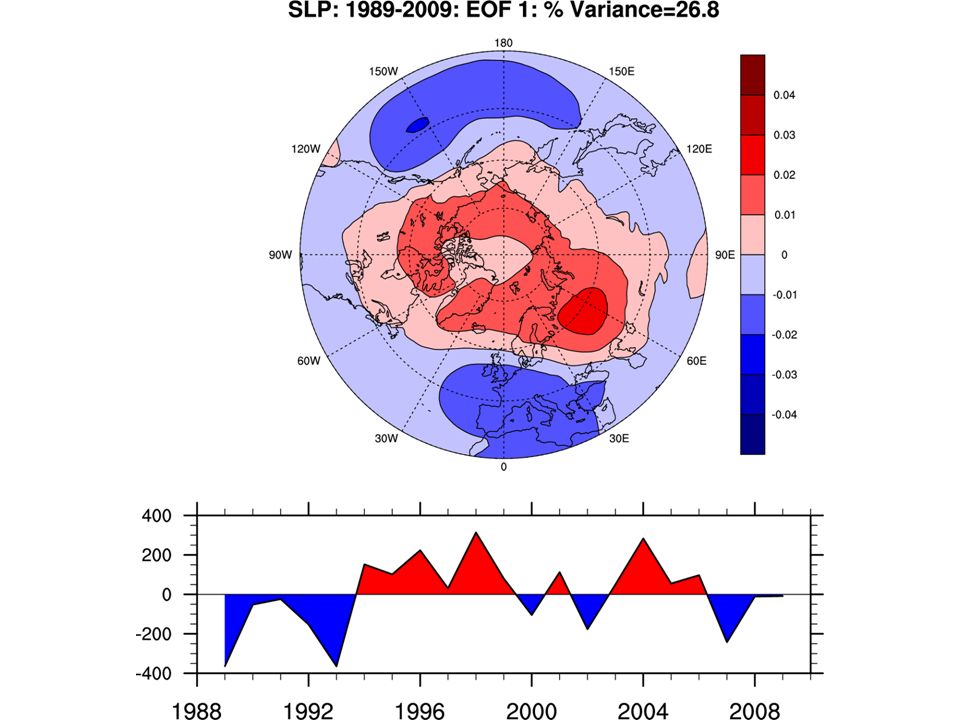


 and the NetCDF Data Format Research Tools Presentation Matthew Janiga 10/30/2012.>")


