1. Pattern recognition – basic concepts

2. Sample input attribute, attribute, feature, input variable, independent variable (atribut, rys, příznak, vstupní proměnná, nezávisle proměnná) class, output variable, dependendent variable (třída, výstupní proměnná, závislá proměnná) sample (vzorek)

3. Handwritten digits

4. each digit 28 x 28 pixels – so each digit can be represented by a vector x comprising 784 real numbers goal: – build a machine that will take x as input and will produce the identity of the digit 0 … 9 as the output – non-trivial problem due to the wide variability of handwriting – could be tackled by using rules for distinguishing the digits based on the shapes of the strokes – in practice such an approach leads to a proliferation of rules and of exceptions to the rules and so on, and invariably gives poor results

5. better way – adopt machine learning algorithm (i.e. use some adaptive model) model input internal parameters influencing the behavior of the model must be adjusted

6. tune the parameters of the model using the training set – training set is a data set of N digits {x 1, …, x N } the categories of the digits in the training set are known in advance (inspected manually), they form a target vector t for each digit (one target vector for each digit) 00010000000123456789

7. The result of running the machine learning algorithm can be expressed as a function y(x) which takes a new digit image x as input and that generates an output vector y, encoded in the same way as the target vectors. y(x) x 784 x6x6 x5x5 x4x4 x3x3 x2x2 x1x1...... vector y

8. The precise form of the function y(x) is determined during the training phase (learning phase). – Model adapts its parameters (i.e. learns) on the basis of the training data {x 1, …, x N }. Trained model can then determine the identity of new, previously unseen, digit images which are said to comprise a test set. The ability to categorize correctly new examples that differ from those used for training is known as generalization.

9. For most practical applications, the original input variables are typically preprocessed to transform them into some new space of variables where, it is hoped, the pattern recognition problem will be easier to solve. y(x) x 784 x6x6 x5x5 x4x4 x3x3 x2x2 x1x1...... vector y Preprocessing

10. Translate and scale the images of the digits so that each digit is contained within a box of a fixed size. This greatly reduces the variability within each digit class, because the location and scale of all the digits are now the same. This pre-processing stage is sometimes also called feature extraction. Test data must be pre-processed using the same steps as the training data.

11. Feature selection and feature extraction x 784 x6x6 x5x5 x4x4 x3x3 x2x2 x1x1...... x 456 x 103 x5x5 x1x1 x 784 x6x6 x5x5 x4x4 x3x3 x2x2 x1x1...... x * 666 x * 309 x * 152 x * 18 x * 784 x*6x*6 x*5x*5 x*4x*4 x*3x*3 x*2x*2 x*1x*1...... selectionextraction

12. Dimensionality reduction We want to reduce number of dimensions because: – Efficiency measurement costs storage costs computation costs – Problem may be solved more easily in the new space – Improved classification performance – Ease of interpretation

13. Curse of dimensionality Bishop, Pattern Recognition and Machine Learning

14. Supervised learning training data comprises examples of the input vectors along with their corresponding target vectors (e.g. digit recognition) – classification – aim: assign an input vector to one of a finite number of discrete categories – regression (data/curve fitting) - desired output consists of one or more continuous variables

15. Unsupervised learning training data consists of a set of input vectors x without any corresponding target value goals: – discover groups of similar examples within the data – clustering – project the data from a high-dimensional space down to two or three dimensions for the purpose of visualization

16. Polynomial curve fitting regression problem, supervised we observe a real-valued input variable x and we wish to use this observation to predict the value of a real-valued target variable t artificial example - sin(2πx n ) + random noise training set: N observations of x written as x = (x 1, …, x N ) T + corresponding observations of the values of t: t = (t 1, …, t N ) T

17. sin(2πx n ) + random noise N = 10 x 1 -> t 1 x 2 -> t 2 etc. training data set {x, t} adapted from Bishop, Pattern Recognition and Machine Learning

18. goal: exploit the training set in order to make prediction of the target variable t’ for new value x’ of the input variable this is generally difficult, as – we have to generalize from the finite data set – data are corrupted by the noise, so for given x’ there is uncertainty in the value of t’ x’ t’ adapted from Bishop, Pattern Recognition and Machine Learning

19. decision: which method to use? From the plethora of possibilities (you do not know about yet) I have chosen a simple one – data will be fitted using this polynomial function polynomial coefficients w 0, …, w M form a vector w – they represent parameters of the model that must be set in the training phase – the polynomial model is still linear regression!!!

20. The values of coefficients will be determined by minimizing the error function It measures the misfit between the function y(x, w) and the training set data points one simple choice: the sum of squared errors - SSE between the predictions y(x n, w) for each data point x n and the correspoding values t n

21. fitted function displacement of the data point t n from the function y(x n, w) Bishop, Pattern Recognition and Machine Learning

22. solving curve fitting problem means choosing the value of w for which E(w) is as small as possible … w* → y(x, w*) – as small as possible means to find a minimum of E(w) (i.e. its derivatives) – However, we already know that in computer this is done by matrix decompositions. Which ones?

23. Model selection overfitting

24. RMS – root mean squared error MSE – mean squared error střední kvadratická chyba comparing error for data sets of different size – root mean squared error RMS

25. Summary of errors sum of squared errors mean squared error root mean squared error

26. Training set Test set

27. the bad result for M = 9 may seem paradoxical because – polynomial of given order contains all lower order polynomials as special cases (M=9 polynomial should be at least as good as M=3 polynomial) OK, let’s examine the values of the coefficients w * for polynomials of various orders

28. M = 0M = 1M = 3M = 9 w0*w0* 0.190.820.310.35 w1*w1* -1.277.99232.37 w2*w2* -25.43-5321.83 w3*w3* 17.3748568.31 w4*w4* -231639.30 w5*w5* 640042.26 w6*w6* -1061800.52 w7*w7* 1042400.18 w8*w8* -557682.99 w9*w9* 125201.43

29. for a given model complexity the overfitting problem becomes less severe as the size of the data set increases M = 9 N = 15 M = 9 N = 100 or in other words, the larger the data set is, the more complex (flexible) model can be fitted

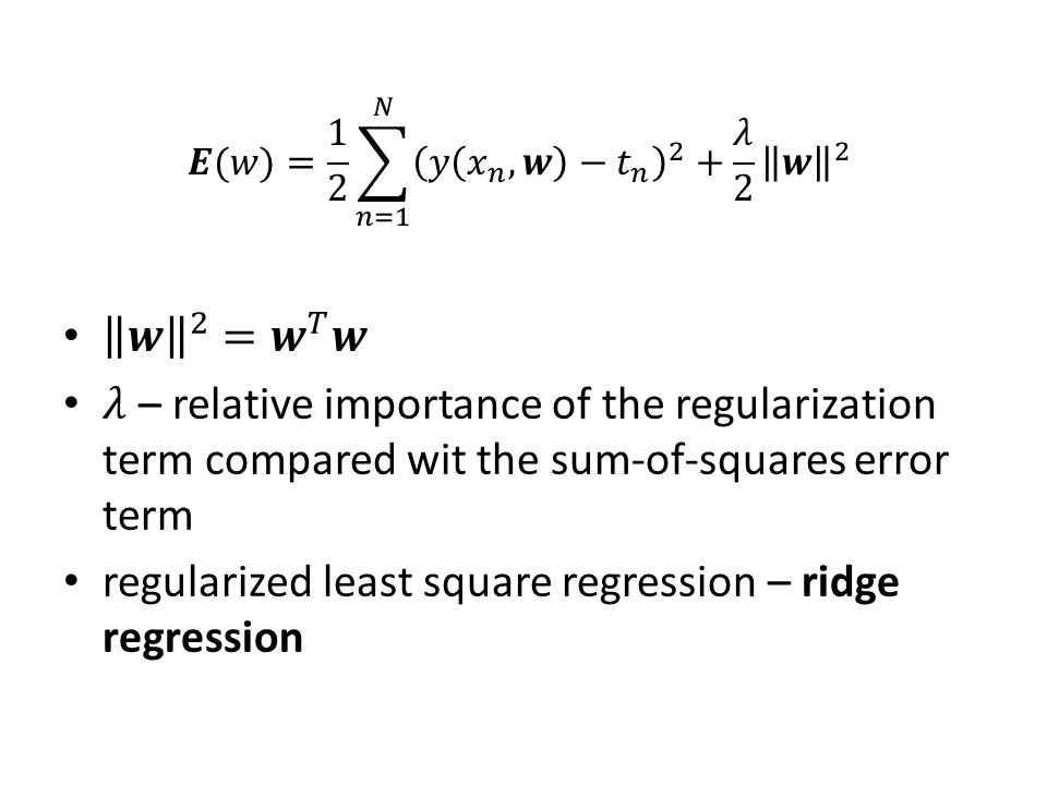
32. ln λ = -∞ln λ = -18ln λ = 0 w0*w0* 0.35 0.13 w1*w1* 232.374.74-0.05 w2*w2* -5321.83-0.77-0.06 w3*w3* 48568.31-31.97-0.05 w4*w4* -231639.30-3.89-0.03 w5*w5* 640042.2655.28-0.02 w6*w6* -1061800.5241.32-0.01 w7*w7* 1042400.18-45.950.00 w8*w8* -557682.99-91.530.00 w9*w9* 125201.4372.680.01 M = 9 N = 10

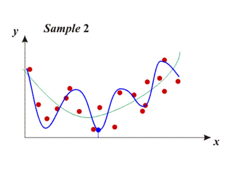
33. Overfitting in classification

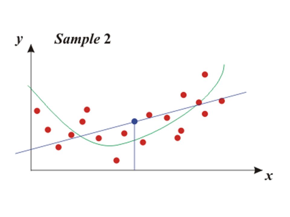
34. Bias-variance tradeoff low flexibility models have large bias and low variance – bias means large quadratic error of the model – variance means that the predictions of the model will depend only little on the particular sample that was used for building the model i.e. there is little change in the model if training data set is changed thus there is little change between predictions for given x for different models

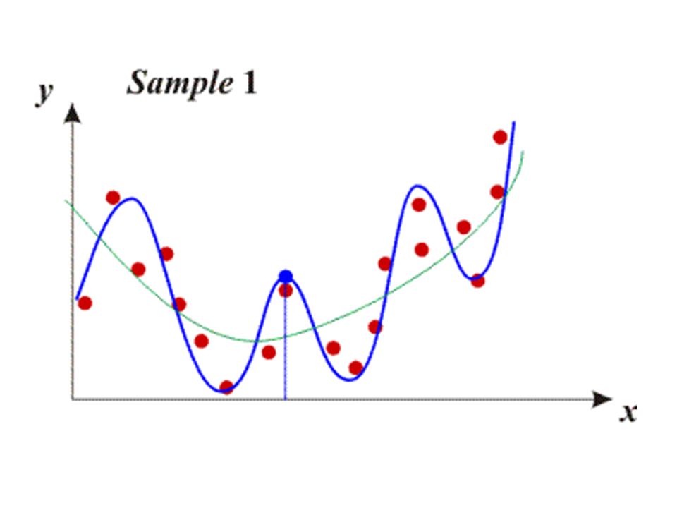
37. high flexibility models have low bias and large variance – Large degree will make the polynomial very sensitive to the details of the sample. – Thus the polynomial changes dramatically upon the change of the data set. – Such a model has large variance because the variance of its predictions (for given x) is large. – However, bias is low, as the quadratic error is low.

40. A polynomial with too few parameters (too low degree) will make large errors because of a large bias. A polynom with too many parameters (too high degree) will make large errors because of a large variance. The degree of the ”best” polynomial must be somewhere ”in-between” - bias-variance tradeoff MSE = variance + bias 2

41. This phenomenon is not specific to polynomial regression! In fact, it shows-up in any kind of model. Generally, the bias-variance tradeoff principle can be stated as: – Models with too few parameters are inaccurate because of a large bias (not enough flexibility). – Models with too many parameters are inaccurate because of a large variance (too much sensitivity to the sample). – Identifying the best model requires identifying the proper “model complexity” (number of parameters).

42. Ende

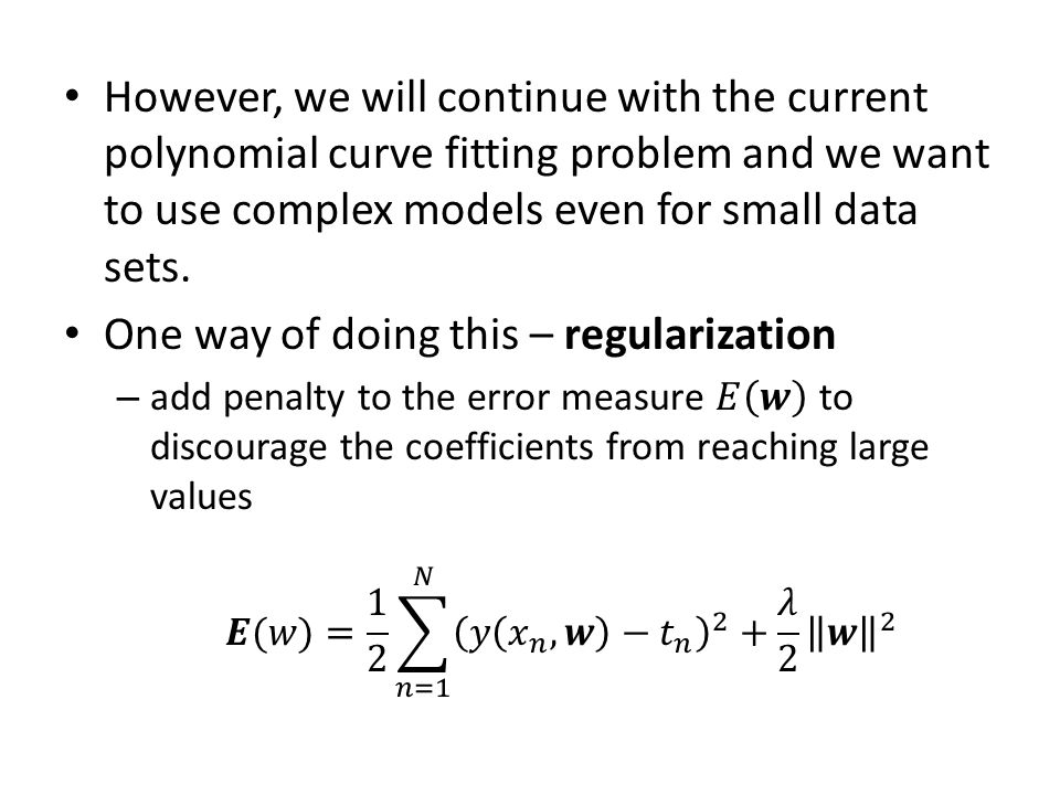
43. However, why should we limit the number of parameters of the model based on the size of the data set? Shouldn’t the complexity of the model be given by the complexity of the problem itself rather than by the number ov available data points? Least squares represents one of the cases of the so-called maximum likelihood approach, for which overfitting is the general property Overfitting can be avoided by adopting Bayesian approach.