1 What is Computer Graphics Computer graphics is commonly understood to mean the creation, storage and manipulation of models and images. (Andries van.

1 What is Computer Graphics Computer graphics is commonly understood to mean the creation, storage and manipulation of models and images. (Andries van Dam) Computer graphic is concerned with - all aspects of producing pictures or images using a computer. - the pictorial synthesis or real or imaginary objects from their computer based model

2 Computer Graphics  Synthesis of graphical images  Visualization : creating an image from an abstract, symbolic description.  Generation of Synthesis Image using graphical primitives data from real world phenomena

3 Image Processing  the transformation of an existing image into a more desirable or useful image. image enhancement The following images represent how noise affects images

4 Image Analysis Image Analysis (Computer Vision)  extracting symbolic information from the image. Computer Graphics Data => Picture Image ProcessingPicture => Picture Image AnalysisPicture => Data

5 What is Interactive Computer Graphics? User controls contents, structure, and appearance of objects and their displayed images via rapid visual feedback Basic components of an interactive graphics system  input (e.g., mouse, tablet and stylus, force feedback device,scanner…)  processing (and storage)  display/output (e.g., screen, paper-based printer, video recorder…)

6 A Brief History teletype printouts were first graphical output devices lightpens were an early input device CAD applications began in the 1960's plotters also a 60's development: high-resolution, but slow main bottlenecks of computer graphics back then cost of graphics hardware expense of computer resources batch systems weren't suitable for interactive graphics non-portability of hardware and software a new field: technology was primitive

7 History of Computer Graphics (1/5) 1950 MIT’s Whirlwind computer had computer generated CRTs mid 1950s SAGE command and control 1960s Ivan Sutherland’s thesis - Sketchpad  introduced data structures and interactive techniques http://www.computer.org/history/development/1951.htm

8 History of Computer Graphics (2/5) 1960s GM (general Motor)  developed CAD (Computer Aided Design) and CAM 1968 Tektronix storage tubes 1970s Boeing CAD CAM

9 Mid 1970s engineering workstations and personal computers emerged separately 1980s new algorithms and techniques  new standards  ever more powerful system  transition from specialized field 1990s widespread use  low cost, but powerful personal workstations  networks  essential part of systems  now part of multimedia History of Computer Graphics (3/5)

10 At first - progress was slow because cost of equipment was high (specially memory) significant computing resources needed difficulty in writing software ( harder than it looks) lack of standard and thus portability lack of software tools History of Computer Graphics (4/5)

11 Now - previous use cost of equipment is low. Most computer have necessary computing resources for graphics established standards, implementations and tools still difficulty in writing software ( still harder than it looks) History of Computer Graphics (5/5)

12 Applications of Computer Graphics divided in 4 majors area  Display of Information  Design  Simulation  User Interface

13 Display of Information Geographic information system (GIS) Computerized Tomography (CT) Magnetic resonance imaging (MRI) Ultrasound http://www.soest.hawaii.edu/soest/about.ftp.html http://www.queens.org/qmc/services/imaging/ct.htm

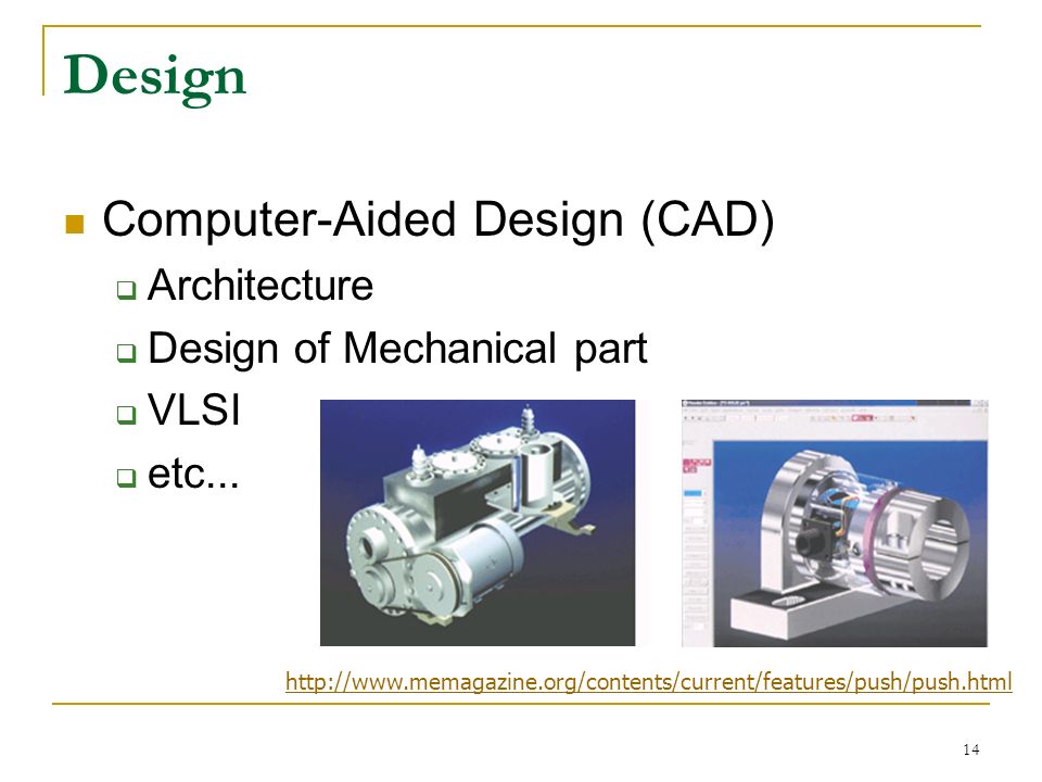
14 Design Computer-Aided Design (CAD)  Architecture  Design of Mechanical part  VLSI  etc... http://www.memagazine.org/contents/current/features/push/push.html

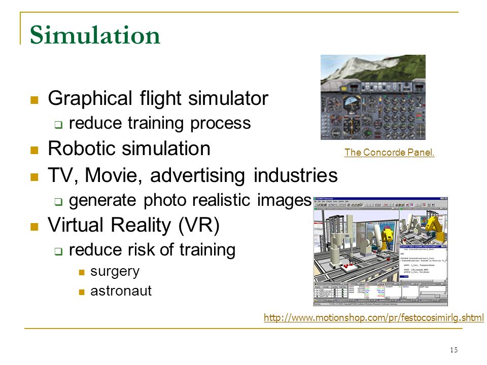
15 Simulation Graphical flight simulator  reduce training process Robotic simulation TV, Movie, advertising industries  generate photo realistic images Virtual Reality (VR)  reduce risk of training surgery astronaut The Concorde Panel. http://www.motionshop.com/pr/festocosimirlg.shtml

16 User Interfaces Window system  Window 2003  X window  MAC OS Graphical Network browsers  Netscape  Internet Explorer

17 Areas of research in Graphics (1/2) mathematical modeling:  interpolation, curve and surface fitting  computational geometry: algorithmic applications in geometry  study of light and optical phenomenon: colour, texture, shades  modelling the characteristics of physical objects (bouncing Jello)

18 Areas of research in Graphics (2/2) Software technology  standardized graphics languages and libraries  graphics tools and interfaces  algorithm design Hardware  specialized graphics chips, monitors, interface devices

19 Graphics Applications (1/5) Entertainment: Cinema Pixar: Geri ’ s Game Universal: Jurassic Park A bug ’ s Life Antz

20 Graphics Applications (2/5) Entertainment: Games Quake III Aki Ross : Final Fantasy Star Wars Jedi Outcast: Jedi Knight II

21 Graphics Applications (3/5) Medical Visualization The Visible Human Project http://www.ercim.org/publication/Ercim_News/enw44/koenig.html

22 Graphics Applications (4/5) Computer Aided Design (CAD)

23 Graphics Applications (5/5) Scientific Visualization

24 Curve and Surface Modeling 1 2 3 4 5 6 7 8 http://www.geocities.com/SiliconValley/Lakes/2057/nurbs.html

25 Photorealistic Illumination Models http://www.pixar.com http://www.ktx.com/3dsmaxr3/ http://www.aliaswavefront.com

26 Fractal Systems http://sprott.physics.wisc.edu/fractals.htm

27 Information Visualization Visible Decisions SeeIT(http://www.vdi.com)

28 Lecture Topics Introduction Mathematical Foundation Coordinate Systems Introduction to Graphics in 2D Windows and Clipping Introduction to Graphics in 3D Viewing in 3D Visible Surface Determination Algorithm efficiency Z-buffer algorithm Scan line algorithms Visible-surface Ray Tracing Other algorithms Color Models Illumination and Shading

29 Mathematical foundation Mathematical appears throughout 3D graphics Example: Object surfaces can be represented as polygons whose vertex position are specified by vectors Rendering requires testing whether vertices lie in front of or behind various planes. The test involves a dot product with the plane’s normal vector.

30 Geometric transformation Goal: specify object’s position and orientations in a 3D world Use Linear transformations that rotate and translate objects’ vertices. Apply these transformations in matrix form

31 Viewing Goal: map the visible part of a 3D world to a 2 D image Use camera-like parameters to define a 3D view volume Project the view voulme onto a 2D image plane Map viewport on the image plane to the screen

32 OpenGL OpenGL is strictly defined as “a software interface to graphics hardware”. It is a 3D graphics and modeling library variety purposes, CAD engineering, architectural applications, computer- generated dianosaurs in blockbuster movies Developed by SGI

33 Clipping Goal: cut off the part of objects outside the view volume to avoid rendering them

34 Scan Conversion Goal: convert a project, clipped object into pixels on raster lines. Use efficient incremental methods

35 Antialiasing Raster displays produce blocky aliasing artifacts Antialiasing techniques reduces the problem by applying the theory of sampling and signal processing

36 Color Various color spaces provide ways to specify colors in term of components: red, green, blue hue, saturation, value Different output devices display different subsets of the perceptible colors

37 Hidden Surface Removal When several overlapping polygons are drawn on the screen, which one is on top? Which is right?

38 Z-buffering A fast hardware solution is the Z-buffer The “depth” of each pixel relative to the screen is calculated and saved in a buffer The pixel with the smallest depth is the one that is displayed The other pixels are on surfaces that are hidden Z Screen This pixel is drawn on screen Polygons

39 Lighting Models and Shading For visual realism, lighting models have been developed to illuminate the surfaces of solid models These models incorporate  ambient lighting and illumination  diffuse reflection of directional lighting  specular reflection of directional lighting Ambient lighting : incident light reflected light incident light reflected light

40 Ray Tracing Ray tracing traces a ray of light from the eye to a light source Ray tracing realistically renders scenes with shiny and transparent objects Eye Light Source Object Light Source Object Shadow Ray Eye Ray

41 Radiosity Diffuse illumination results from the absorption and reflection of diffuse light from many objects in the scene Radiosity uses thermal models of emission and reflection of radiation to accurately calculate diffuse lighting Radiosity is very good at rendering architectural interiors

42 Texture Mapping For realism, photographic textures are “mapped” onto the surfaces of objects Example textures:  woodgrain  concrete  grass  marble Texture mapping is very computationally intensive shadows texture mapping reflections

43 Example of Shading WireframeFlat Shaded Smooth Shaded Shadows

44 Mathematical Foundation for Graphics

45 Objectives Introduce the elements of geometry  Scalars  Vectors  Points Develop mathematical operations among them in a coordinate-free manner Define basic primitives  Line segments  Polygons

46 Basic Elements Geometry is the study of the relationships among objects in an n-dimensional space  In computer graphics, we are interested in objects that exist in three dimensions Want a minimum set of primitives from which we can build more sophisticated objects We will need three basic elements  Scalars  Vectors  Points

47 Coordinate-Free Geometry When we learned simple geometry, most of us started with a Cartesian approach  Points were at locations in space p=(x,y,z)  We derived results by algebraic manipulations involving these coordinates This approach was nonphysical  Physically, points exist regardless of the location of an arbitrary coordinate system  Most geometric results are independent of the coordinate system  Euclidean geometry: two triangles are identical if two corresponding sides and the angle between them are identical

48 Geometry Geometry provides a mathematical foundation for much of computer graphics:  Geometric Spaces: Vector, Affine, Euclidean, Cartesian, Projective  Affine Geometry  Affine Transformations  Perspective  Projective Transformations  Matrix Representation of Transformations  Viewing Transformations

49 Introduction (1/2) Points are associated with locations of space Vectors represent displacements between points or directions Points, vectors, and operators that combine them are the common tools for solving many geometric problems that arise in Geometric Modeling, Computer Graphics, Animation, Visualization, and Computational Geometry.

50 Introduction (2/2) The three most fundamental operators on vectors are the dot product, the cross product, and the mixed product (sometimes called the triple product). Although a point and a vector may be represented by its three coordinates, they are of different type and should not be mixed

51 What will you learn here? (1/2) Properties of dot, cross, and mixed products How to write simple tests for  4-points and 2-lines coplanarity  Intersection of two coplanar edges  Parallelism of two edges or of two lines  Clockwise orientation of a triangle from a viewpoint  Positive orientation of a tetrahedron  Edge/triangle and ray/triangle intersection

52 What will you learn here? (2/2) How to compute  Center of mass of a triangle  Volume of a tetrahedron  “ Shadow ” (orthogonal projection) of a vector on a plane  Line/plane intersection  Plane/plane intersection  Plane/plane/plane intersection

53 Terminology Orthogonal to = Normal to = forms a 90 o angle with Norm of a vector = length of the vector Are coplanar = there is a plane containing them

54 Notation  means “is always equal to” or “by definition” == means the test “is equal to” used in Boolean expressions := is the assignment “is computed as” and is used in construction algorithms s (italic type) Boolean v (normal type) scalar a (bold type lower-case) point A A (bold upper-case) pointset (edge, curve, triangle, surface, solid) U (bold underscored upper-case) vector u (bold underscored lower-case) unit vector T (bold upper-case) transformation

55 Scalars Need three basic elements in geometry  Scalars, Vectors, Points Scalars can be defined as members of sets which can be combined by two operations (addition and multiplication) obeying some fundamental axioms (associativity, commutivity, inverses) Examples include the real and complex number systems under the ordinary rules with which we are familiar Scalars alone have no geometric properties

56 Vectors And Point We commonly use vectors to represent:  Points in space (i.e., location)  Displacements from point to point  Direction (i.e., orientation) But we want points and directions to behave differently  Ex: To translate something means to move it without changing its orientation  Translation of a point = different point  Translation of a direction = same direction

57 Vectors Physical definition: a vector is a quantity with two attributes  Direction  Magnitude Examples include  Force  Velocity  Directed line segments Most important example for graphics Can map to other types v

58 Vector Operations Every vector has an inverse  Same magnitude but points in opposite direction Every vector can be multiplied by a scalar There is a zero vector  Zero magnitude, undefined orientation The sum of any two vectors is a vector  Use head-to-tail axiom v -v vv v u w

59 Vectors Lack Position These vectors are identical  Same direction and magnitude Vectors spaces insufficient for geometry  Need points

60 Vectors (1/2) Vector space (analytic definition from Descartes in the 1600s)  U+V=V+U (vector addition)  U+(V+W)=(U+V)+W  0 is the zero (or null) vector if  V, 0+V=V  –V is the inverse of V, so that the vector subtraction V–V= 0  s(U+V)=sU+sV (scalar multiplication)  U/s is the scalar division (same as multiplication by s –1 ) i.e. U/s = s –1 U  (a+b)V=aV+bV

61 Vectors (2/2) Vectors are used to represent displacement between points  Each vector V has a norm (length) denoted ||V||  Let assume V = (v 1,v 2,v 3, …,v n ), ||V|| = | V | =  V / ||V|| is the unit vector (length 1) of V. We denote it V u or v  If ||V||==0, then V is the null vector 0  Unit vectors are used to represent  Basis vectors of a coordinate system  Directions of tangents or normals in definitions of lines or planes

62 Vector Spaces A linear combination of vectors results in a new vector: v =  1 v 1 +  2 v 2 + … +  n v n where  is any scalar If the only set of scalars such that  1 v 1 +  2 v 2 + … +  n v n = 0 is  1 =  2 = … =  3 = 0 then we say the vectors are linearly independent The dimension of a space is the greatest number of linearly independent vectors possible in a vector set For a vector space of dimension n, any set of n linearly independent vectors form a basis

63 Vector Spaces: An Example  Vectors are “ arrows ” rooted at the origin  Scalar multiplication “ streches ” the arrow, changing its length (magnitude) but not its direction  Addition uses the “ trapezoid rule ” : u+v y x u v

64 Points Location in space Operations allowed between points and vectors  Point-point subtraction yields a vector  Equivalent to point-vector addition P = v + Q v = P - Q

65 Affine Spaces Point + a vector space Operations  Vector-vector addition  Scalar-vector multiplication  Point-vector addition  Scalar-scalar operations For any point define  1 P = P  0 P = 0 (zero vector)

66 Affine Space (1/2) Definition: Set of Vectors V and a Set of Points P Vectors V form a vector space. Points can be combined with vectors to make new points: P + v =Q with P,Q  P and v  V Dimension: The dimension of an affine space is the same as that of V.

67 Affine Space (2/2) Note:  All other point operations are just variations on the P + v operation.  No distinguished origin  No notion of distances or angles.  Most of what we do in graphics is affine.

68 Affine space V=b–a (vector V is the displacement from point a to point b)  Notation: ab stands for the vector b – a  c– a = (c – b) + (b – a). Written ac = ab + bc  Point b is uniquely defined, given point a and vector (b – a)

69 Affine space  Points may be used to represent  The vertices of a triangle or polyhedron  The origin of a coordinate system  Points in the definition of lines or plane

70 Lines Consider all points of the form  P(  )=P 0 +  d  Set of all points that pass through P 0 in the direction of the vector d

71 Parametric Form This form is known as the parametric form of the line  More robust and general than other forms  Extends to curves and surfaces Two-dimensional forms  Explicit: y = mx +h  Implicit: ax + by +c =0  Parametric: x(  ) =  x 0 + (1-  )x 1 y(  ) =  y 0 + (1-  )y 1

72 Rays and Line Segments If  >= 0, then P(  ) is the ray leaving P 0 in the direction d If we use two points to define v, then P(  ) = Q+  v = Q +  (R-Q) =  R + (1-  )Q For 0<=  <=1 we get all the points on the line segment joining R and Q

73 Convexity An object is convex iff for any two points in the object all points on the line segment between these points are also in the object P Q Q P convex not convex

74 Affine Sums Consider the “ sum ” P=  1 P 1 +  2 P 2 +…..+  n P n Can show by induction that this sum makes sense iff  1 +  2 + …..  n =1 in which case we have the affine sum of the points P 1  P 2,…..P n If, in addition,  i >=0, we have the convex hull of P 1  P 2,…..P n

75 Convex Hull Smallest convex object containing P 1  P 2,…..P n Formed by “ shrink wrapping ” points

76 Curves and Surfaces Curves are one parameter entities of the form P(  ) where the function is nonlinear Surfaces are formed from two-parameter functions P( ,  )  Linear functions give planes and polygons P(  ) P( ,  )

77 Planes A plane be determined by a point and two vectors or by three points P( ,  )=R+  u+  v P( ,  )=R+  (Q-R)+  (P-Q)

78 Triangles convex sum of P and Q convex sum of S(  ) and R for 0<= ,  <=1, we get all points in triangle

79 Normals Every plane has a vector n normal (perpendicular, orthogonal) to it From point-two vector form P( ,  )=R+  u+  v, we know we can use the cross product to find n = u  v and the equivalent form (P(  )-P)  n=0 u v P

80 Dot Product (1/2) U  V denotes the dot product (also called the inner product) U  V = ||U||  ||V||  cos(angle(U,V))  U  V is a scalar.  U  V==0  ( U==0 or V==0 or (U and V are orthogonal)) u v cos(angle(u,v)) V  U = U  V < 0 hereV  U = U  V > 0 here

81 Dot Product (2/2)  U  V is positive if the angle between U and V is less than 90 o  Note that U  V = V  U, because: cos(a)=cos(– a).  u  v = cos(angle(u,v) # unit vectors: ||u||  1  the dot product of two unit vectors is the cosine of their angle  V  u = length of the orthogonal projection of V onto the direction of u  ||U||= sqrt(U  U) = length of U = norm of U

82 Dot Product The dot product or, more generally, inner product of two vectors is a scalar: v 1 v 2 = x 1 x 2 + y 1 y 2 + z 1 z 2 (in 3D) Useful for many purposes  Computing the length of a vector: length( v ) = sqrt( v v)  Normalizing a vector, making it unit-length  Computing the angle between two vectors: u v = |u| |v| cos(θ)  Checking two vectors for orthogonality  Projecting one vector onto another θ u v

83 Given the unit normal n to a mirror surface and the unit direction l towards the light, compute the direction r of the reflected light. Computing the reflection vector n l r By symmetry, l+r is parallel to n and has a norm that is twice the length of the projection n  l of l upon n. Hence: r = 2(n  l)n–l l r –l–l

84 Computing a “ shadow ” vector (projection) Given the unit up-vector u and the unit direction d, compute the shadow T of d onto the floor (orthogonal to u). T and u are orthogonal. d is the vector sum T+ ( d  u )u. Hence: T = d – (du)uT = d – (du)u u d T

85 Cross product (1/3) U  V denotes the cross product U  V is either 0 or a vector orthogonal to both U and V When U==0 or V==0 or U//V (parallel) then U  V= 0 Otherwise, U  V is orthogonal to both U and V

86 Cross product (2/3) The direction of U  V is defined by the thumb of the right hand Curling the fingers from U to V  Or standing parallel to U and looking at V, U  V goes left ||U  V||  ||U||  ||V||  sin(angle(U,V)) sin(angle(u,v) 2  1 – (u  v) 2 # unit vectors (u  v== 0)  u//v (parallel) U  V  – V  U Useful identity: U  (V  W)  (U  W)V – (U  V)W

87 Cross Product (3/3) The cross product or vector product of two vectors is a vector: The cross product of two vectors is orthogonal to both Right-hand rule dictates direction of cross product

88 When are two edges parallel in 3D? Edge(a,b) is parallel to Edge(c,d) if ab  cd == 0

89 Mixed product U  ( V  W ) is called a mixed product  U  (V  W) is a scalar  U  (V  W) ==0 when one of the vectors is null or all 3 are coplanar  U  (V  W) is the determinant | U V W |  U  (V  W)  V  (W  U)  – U  (W  V) # cyclic permutation

90 Testing whether a triangle is front-facing When does the triangle a, b, c appear clockwise from d? when da  (db  dc) > 0 a b c d

91 Volume of a tetrahedron Volume of a tetrahedron with vertices a, b, c and d is v  | da  (db  dc) | / 6 db c dc db db  dc a da

92 z, s, and v functions (1/2) zero: z(a,b,c,d)  da  (db  dc)==0 # tests co-planarity of 4 points  Returns Boolean TRUE when a,b,c,d are coplanar sign: s(a,b,c,d)  da  (db  dc)>0 # test orientation or side  Returns Boolean TRUE when a,b,c appear clockwise from d  Used to test whether d in on the “good” side of plane through a,b,c db c dc db db  dc a da c a b d

93 z, s, and v functions (2/2) value: v(a,b,c,d)  da  (db  dc) # compute volume  Returns scalar whose absolute value is 6 times the volume of tetrahedron a,b,c,d  v(a,b,c,d)  v(d,a,b,c)  –v(b,a,c,d)

94 Testing whether an edge is concave How to test whether the edge (c,b) shared by triangles (a,b,c) and (c,b,d) is concave?

95 When do two edges intersect in 2D? Write a geometric expression that returns true when two coplanar edges (a,b) and (c,d) intersect a b d c 0  (ab  ac)(ab  ad) and 0  (cd  ca)(cd  cb) d c a b

96 When do two edges intersect in 3D? Consider two edges: edge(a,b) and edge(c,d) When are they co-planar? When do they intersect? a b d c q p When z(a,b,c,d) When they are co-planar and 0  (ab  ac)(ab  ad) and 0  (cd  ca)(cd  cb) a b d c

97 What is the common normal to 2 edges in 3D? Consider two edges: edge(a,b) and edge(c,d) What is their common normal n? a b d c n n=(ab  cd) u

98 When is a point inside a tetrahedron? When does point p lie inside tetrahedron a, b, c, d ?  Assume z(a,b,c,d) is FALSE (not coplanar) When is p on the boundary of the tetrahedron?  Do as an exercise for practice. ba c p d When s(a,b,c,d), s(p,b,c,d), s(a,p,c,d), s(a,b,p,d), and s(a,b,c,p) are identical. (i.e. all return TRUE or all return FALSE)

99 A faster point-in-tetrahedron test ? Suggested by Nguyen Truong  Write ap = sab+tac+uad  Solve for s, t, u (linear system of 3 equations)  Requires 17 multiplications, 3 divisions, and 11 additions  Check that s, t, and u are positive and that s+u+t<1 A more expensive Variation: Compute s, t, u, w  w = v(a,b,c,d)  s = v(a,p,c,d)  u = v(a,b,p,d)  t = v(a,b,c,p) Check that  w, s, t, u have the same sign and that s+u+t<w ba c p d

100 When is a 3D point inside a triangle When does point p lie inside triangle with vertices a, b, c ? a b c p p When z(p,a,b,c) and (ab  ap)(bc  bp)  0 and (bc  bp)(ca  cp)  0

101 Parametric representation of a line Let Line(p,t) be the line through point p with tangent t Its parametric form associates a scalar s with a point q(s) on the line s defines the distance from p to q(s) q(s) = p + st  Note that the direction of t gives an orientation to the line (direction where s is positive) We can represent a line by p and t p q t s

102 Implicit representation of a plane Let Plane(r,n) be the plane through point r with normal n Its implicit form states that a point q lies on Plane(r,n) when rq  n=0  Remember that rq = q – r Note that the direction of n defines an orientation of the plane p n r q n r p not in plane

103 Line/plane intersection Compute the point q of intersection between Line(p,t) and Plane(r,n) Replacing q by p+st in (q–r)  n=0 yields (p–r+st)  n=0 Solving for s yields rp  n+st  n=0 and s = – rp  n / t  n s = pr  n / t  n Hence q = p + (pr  n)t / (t  n) p q t n r s

104 When are two lines coplanar in 3D? L(p,t) and L(q,u) are coplanar When t  u == 0 OR pq(t  u) == 0

105 What is the intersection of two planes Consider two planes Plane(p,n) and Plane(q,m) Assume that n and m are not parallel (i.e. n  m ≠ 0) Their intersection is a line Line(r,t). How can one compute r and t ? t := (n  m) u let u := n  t r := p+( pqm)u /(um) q p n m r u t If correct, then provide the derivation. Otherwise, provided the correct answer.

106 What is the intersection of three planes Consider planes Plane(p,m), Plane(q,n), and Plane(r,m). How do you compute their intersection w ? q p n m r t w Write w=p+an+bm+ct then solve the linear system {pwn=0, qwm=0, rwt=0} for a, b, and c or compute the line of intersection between two of these planes and then intersect it with the third one.

107 Implementation Points and vectors are each represented by their 3 coordinates  p=(p x,p y,p z ) and v=(v x,v y,v z ) U V = U x V x + U y V y + U z V z U  V = (U y V z – U z V y ) – (U x V z – U z V x ) + (U x V y – U y V x ) Implement:  Points and vectors  Dot, cross, and mixed products  z, s, and v functions from mixed products  Edge/triangle intersection  Lines and Planes  Line/Plane, Plane/Plane, and Plane/Plane/Plane intersections Return exception for singular cases (parallelism … )

108 Linear Transformations A linear transformation:  Maps one vector to another  Preserves linear combinations Thus behavior of linear transformation is completely determined by what it does to a basis Turns out any linear transform can be represented by a matrix

109 Matrices By convention, matrix element M rc is located at row r and column c: By (OpenGL) convention, vectors are columns:

110 Matrices Matrix-vector multiplication applies a linear transformation to a vector: Recall how to do matrix multiplication

111 Matrix Transformations A sequence or composition of linear transformations corresponds to the product of the corresponding matrices  Note: the matrices to the right affect vector first  Note: order of matrices matters! The identity matrix I has no effect in multiplication Some (not all) matrices have an inverse:

112 2D and 3D Transformation

113 Transformations and Matrices Transformations are functions Matrices are functions representations Matrices represent linear transformation {2x2 Matrices}  {2D Linear Transformation}

114 Transformations (1/3) What are they?  changing something to something else via rules  mathematics: mapping between values in a range set and domain set (function/relation)  geometric: translate, rotate, scale, shear,… Why are they important to graphics?  moving objects on screen / in space  mapping from model space to screen space  specifying parent/child relationships  …

115 Transformation (2/3) Translation  Moving an object Scale  Changing the size of an object tyty txtx w old w new h old h new x new = x old + t x ; y new = y old + t y s x =w new /w old s y =h new /h old x new = s x x old y new = s y y old

116 Transformation (3/3) To rotate a line or polygon, we must rotate each of its vertices Shear (x,y) Original Datay Shear x Shear

117 What is a 2D Linear Transform? Example

118 Example Scale in x by 2

119 Transformations: Translation (1/2) A translation is a straight line movement of an object from one position to another. A point (x,y) is transformed to the point (x’,y’) by adding the translation distances T x and T y : x’ = x + T x y’ = y + T y

120 Transformations: Translation(2/2) moving a point by a given t x and t y amount e.g. point P is translated to point P’ moving a line by a given t x and t y amount translate each of the 2 endpoints

121 Transformations: Rotation (1/4) Objects rotated according to angle of rotation theta (  ) Suppose a point P(x,y) is transformed to the point P'(x',y') by an anti-clockwise rotation about the origin by an angle of  degrees, then: Given x = r cos , y = r sin  x’ = x cos  – y sin  y’ = y sin  + y cos 

122 Transformations: Rotation (2/4) Rotation P by  anticlockwise relative to origin (0,0)

123 Transformations: Rotation (3/4) Rotation about an arbitary pivot point (x R,y R ) Step 1: translation of the object by (-x R,-y R ) x 1 = x - x R y 1 = y - y R Step 2: rotation about the origin x 2 = x 1 cos(  ) - y 1 sin (  ) y 2 = y 1 cos(  ) - x 1 sin (  ) Step 3: translation of the rotated object by (xR,yR) x’ = x r + x 2 y’ = y r + y 2

124 Transformations: Rotation (4/4) object can be rotated around an arbitrary point (x r,y r ) known as rotation or pivot point by: x' = x r + (x - x r ) cos(  ) - (y - y r ) sin (  ) y' = y r + (x - x r ) sin (  )+(y - y r ) cos(  )

125 Transformations: Scaling (1/5) Scaling changes the size of an object Achieved by applying scaling factors s x and s y Scaling factors are applied to the X and Y co-ordinates of points defining an object’s

126 Transformations: Scaling (2/5) uniform scaling is produced when s x and s y have same valuei.e. s x = s y non-uniform scaling is produced when s x and s x are not equal - e.g. an ellipse from a circle.  i.e. s x  s y x 2 = s x x 1 y 2 = s y y 1

127 Transformations: Scaling (3/5) Simple scaling - relative to (0,0) General form: Ex: s x = 2 and s y =1

128 Transformations: Scaling (4/5) If the point (x f,y f ) is to be the fixed point, the transformation is: x' = x f + (x - x f ) S x y' = y f + (y - y f ) S y This can be rearranged to give: x' = x S x + (1 - S x ) x f y' = y S y + (1 - S y ) y f which is a combination of a scaling about the origin and a translation.

129 Transformations: Scaling (5/5)

130 Transformation as Matrices Scale: x’ = s x x y’ = s y y Rotation: x’ = xcos  - ysin  y’ = xsin  + ycos  Translation: x’ = x + t x y’ = y + t y

131 Transformations: Shear (1/2) Shear in x:

132 Transformations: Shear (2/2) Shear in y:

133 Shear in x then in y

134 Shear in y then in x

135 Homogeneous coordinate As translations do not have a 2 x 2 matrix representation, we introduce homogeneous coordinates to allow a 3 x 3 matrix representation. The Homogeneous coordinate corresponding to the point (x,y) is the triple (x h, y h, w) where: x h = wx y h = wy For the two dimensional transformations we can set w = 1.

136 Matrix representation

137 Basic Transformation (1/3) Translation

138 Basic Transformation (2/3) Rotation

139 Basic Transformation (3/3) Scaling

140 Composite Transformation Suppose we wished to perform multiple transformations on a point:

141 Example of Composite Transformation(1/3) A scaling transformation at an arbitrary angle is a combination of two rotations and a scaling: R(-t) S(S x,S y ) R(t) A rotation about an arbitrary point (x f,y f ) by and angle t anti-clockwise has matrix: T(-x f,-y f ) R(t) T(x f,y f )

142 Example of Composite Transformation(2/3) Reflection about the y-axisReflection about the x-axis

143 Example of Composite Transformation(3/3) Reflection about the originReflection about the line y=x

144 3D Transformation Z X Y Y X Z

145 Basic 3D Transformations Translation Scale Rotation Shear As in 2D, we use homogeneous coordinates (x,y,z,w), so that transformations may be composited together via matrix multiplication.

146 3D Translation and Scaling TP = (x + t x, y + t y, z + t z ) SP = (s x x, s y y, s z z)

147 3D Rotation (1/4) Positive Rotations are defined as follows: Axis of rotation is Direction of positive rotation is xy to z yz to x zx to y

148 3D Rotation (2/4) Rotation about x-axis R x ( ß )P

149 3D Rotation (3/4) Rotation about y-axis R y ( ß )P

150 3D Rotation (4/4) Rotation about z-axis R z (ß)P

151 3D Shear xy Shear: SH xy P

152 Rotation About An Arbitary Axis (1/3) 1. Translate one end of the axis to the origin 2. Rotate about the y- axis and angle  3. Rotate about the x- axis through an angle  Z P1P1 P2P2 Y X b a c u1u1 u2u2 u3u3 ß U

153 Rotation About An Arbitary Axis (2/3) Z P1P1 P2P2 Y X b a c u1u1 u2u2 u3u3 ß U Z Y X b a c u1u1 u2u2 u3u3 ß U Z Y µ a u2u2 X R 4. When U is aligned with the z-axis, apply the original rotation, R, about the z-axis. 5. Apply the inverses of the transformations in reverse order.

154 Rotation About An Arbitary Axis (3/3) T -1 R y ( ß ) R x (- µ ) R R x ( µ ) R y (- ß ) T P

Hierarchical Modeling

156 Angel: Interactive Computer Graphics 3E © Addison-Wesley 2002 Objectives Examine the limitations of linear modeling  Symbols and instances Introduce hierarchical models  Articulated models  Robots Introduce Tree and DAG models

157 Angel: Interactive Computer Graphics 3E © Addison-Wesley 2002 Instance Transformation Start with a prototype object (a symbol) Each appearance of the object in the model is an instance  Must scale, orient, position  Defines instance transformation

158 Angel: Interactive Computer Graphics 3E © Addison-Wesley 2002 Symbol-Instance Table Can store a model by assigning a number to each symbol and storing the parameters for the instance transformation

159 Angel: Interactive Computer Graphics 3E © Addison-Wesley 2002 Relationships in Car Model Symbol-instance table does not show relationships between parts of model Consider model of car  Chassis + 4 identical wheels  Two symbols Rate of forward motion determined by rotational speed of wheels

160 Angel: Interactive Computer Graphics 3E © Addison-Wesley 2002 Structure Through Function Calls car(speed) { chassis() wheel(right_front); wheel(left_front); wheel(right_rear); wheel(left_rear); } Fails to show relationships well Look at problem using a graph

161 Angel: Interactive Computer Graphics 3E © Addison-Wesley 2002 Graphs Set of nodes and edges (links) Edge connects a pair of nodes  Directed or undirected Cycle: directed path that is a loop loop

162 Angel: Interactive Computer Graphics 3E © Addison-Wesley 2002 Tree Graph in which each node (except the root) has exactly one parent node  May have multiple children  Leaf or terminal node: no children root node leaf node

163 Angel: Interactive Computer Graphics 3E © Addison-Wesley 2002 Tree Model of Car

164 Angel: Interactive Computer Graphics 3E © Addison-Wesley 2002 DAG Model If we use the fact that all the wheels are identical, we get a directed acyclic graph  Not much different than dealing with a tree

165 Angel: Interactive Computer Graphics 3E © Addison-Wesley 2002 Modeling with Trees Must decide what information to place in nodes and what to put in edges Nodes  What to draw  Pointers to children Edges  May have information on incremental changes to transformation matrices (can also store in nodes)

166 Angel: Interactive Computer Graphics 3E © Addison-Wesley 2002 Robot Arm robot arm parts in their own coodinate systems

167 Angel: Interactive Computer Graphics 3E © Addison-Wesley 2002 Articulated Models Robot arm is an example of an articulated model  Parts connected at joints  Can specify state of model by giving all joint angles

168 Angel: Interactive Computer Graphics 3E © Addison-Wesley 2002 Relationships in Robot Arm Base rotates independently  Single angle determines position Lower arm attached to base  Its position depends on rotation of base  Must also translate relative to base and rotate about connecting joint Upper arm attached to lower arm  Its position depends on both base and lower arm  Must translate relative to lower arm and rotate about joint connecting to lower arm

169 Angel: Interactive Computer Graphics 3E © Addison-Wesley 2002 Required Matrices Rotation of base: R b  Apply M = R b to base Translate lower arm relative to base: T lu Rotate lower arm around joint: R lu  Apply M = R b T lu R lu to lower arm Translate upper arm relative to upper arm: T uu Rotate upper arm around joint: R uu  Apply M = R b T lu R lu T uu R uu to upper arm

170 Angel: Interactive Computer Graphics 3E © Addison-Wesley 2002 OpenGL Code for Robot robot_arm() { glRotate(theta, 0.0, 1.0, 0.0); base(); glTranslate(0.0, h1, 0.0); glRotate(phi, 0.0, 1.0, 0.0); lower_arm(); glTranslate(0.0, h2, 0.0); glRotate(psi, 0.0, 1.0, 0.0); upper_arm(); }

171 Angel: Interactive Computer Graphics 3E © Addison-Wesley 2002 Tree Model of Robot Note code shows relationships between parts of model  Can change “look” of parts easily without altering relationships Simple example of tree model Want a general node structure for nodes

172 Angel: Interactive Computer Graphics 3E © Addison-Wesley 2002 Possible Node Structure Code for drawing part or pointer to drawing function linked list of pointers to children matrix relating node to parent

173 Angel: Interactive Computer Graphics 3E © Addison-Wesley 2002 Generalizations Need to deal with multiple children  How do we represent a more general tree?  How do we traverse such a data structure? Animation  How to use dynamically?  Can we create and delete nodes during execution?

Hierarchical Modeling II

175 Angel: Interactive Computer Graphics 3E © Addison-Wesley 2002 Objectives Build a tree-structured model of a humanoid figure Examine various traversal strategies Build a generalized tree-model structure that is independent of the particular model

176 Angel: Interactive Computer Graphics 3E © Addison-Wesley 2002 Humanoid Figure

177 Angel: Interactive Computer Graphics 3E © Addison-Wesley 2002 Building the Model Can build a simple implementation using quadrics: ellipsoids and cylinders Access parts through functions  torso()  left_upper_arm() Matrices describe position of node with respect to its parent  M lla positions left lower leg with respect to left upper arm

178 Angel: Interactive Computer Graphics 3E © Addison-Wesley 2002 Tree with Matrices

179 Angel: Interactive Computer Graphics 3E © Addison-Wesley 2002 Display and Traversal The position of the figure is determined by 11 joint angles (two for the head and one for each other part) Display of the tree requires a graph traversal  Visit each node once  Display function at each node that describes the part associated with the node, applying the correct transformation matrix for position and orientation

180 Angel: Interactive Computer Graphics 3E © Addison-Wesley 2002 Transformation Matrices There are 10 relevant matrices  M positions and orients entire figure through the torso which is the root node  M h positions head with respect to torso  M lua, M rua, M lul, M rul position arms and legs with respect to torso  M lla, M rla, M lll, M rll position lower parts of limbs with respect to corresponding upper limbs

181 Angel: Interactive Computer Graphics 3E © Addison-Wesley 2002 Stack-based Traversal Set model-view matrix to M and draw torso Set model-view matrix to MM h and draw head For left-upper arm need MM lua and so on Rather than recomputing MM lua from scratch or using an inverse matrix, we can use the matrix stack to store M and other matrices as we traverse the tree

182 Angel: Interactive Computer Graphics 3E © Addison-Wesley 2002 Traversal Code figure() { glPushMatrix() torso(); glRotate3f(…); head(); glPopMatrix(); glPushMatrix(); glTranslate3f(…); glRotate3f(…); left_upper_arm(); glPopMatrix(); glPushMatrix(); save present model-view matrix update model-view matrix for head recover original model-view matrix save it again update model-view matrix for left upper arm recover and save original model-view matrix again rest of code

183 Angel: Interactive Computer Graphics 3E © Addison-Wesley 2002 Analysis The code describes a particular tree and a particular traversal strategy  Can we develop a more general approach? Note that the sample code does not include state changes, such as changes to colors  May also want to use glPushAttrib and glPopAttrib to protect against unexpected state changes affecting later parts of the code

184 Angel: Interactive Computer Graphics 3E © Addison-Wesley 2002 General Tree Data Structure Need a data structure to represent tree and an algorithm to traverse the tree We will use a left-child right sibling structure  Uses linked lists  Each node in data structure is two pointers  Left: next node  Right: linked list of children

185 Angel: Interactive Computer Graphics 3E © Addison-Wesley 2002 Left-Child Right-Sibling Tree

186 Angel: Interactive Computer Graphics 3E © Addison-Wesley 2002 Tree node Structure At each node we need to store  Pointer to sibling  Pointer to child  Pointer to a function that draws the object represented by the node  Homogeneous coordinate matrix to multiply on the right of the current model-view matrix Represents changes going from parent to node In OpenGL this matrix is a 1D array storing matrix by columns

187 Angel: Interactive Computer Graphics 3E © Addison-Wesley 2002 C Definition of treenode typedef struct treenode { Glfloat m[16]; void (*f)(); struct treenode *sibling; struct treenode *child; } treenode;

188 Angel: Interactive Computer Graphics 3E © Addison-Wesley 2002 Defining the torso node treenode torso_node, head_node, lua_node, … ; /* use OpenGL functions to form matrix */ glLoadIdentity(); glRotatef(theta[0], 0.0, 1.0, 0.0); /* move model-view matrix to m */ glGetFloatv(GL_MODELVIEW_MATRIX, torso_node.m) torso_node.f = torso; /* torso() draws torso */ Torso_node.sibling = NULL; Torso_node.child = &head_node;

189 Angel: Interactive Computer Graphics 3E © Addison-Wesley 2002 Notes The position of figure is determined by 11 joint angles stored in theta[11] Animate by changing the angles and redisplaying We form the required matrices using glRotate and glTranslate  More efficient than software  Because the matrix is formed in model-view matrix, we may want to first push original model- view matrix on matrix stach

190 Angel: Interactive Computer Graphics 3E © Addison-Wesley 2002 Preorder Traversal void traverse(treenode *root) { if(root == NULL) return; glPushMatrix(); glMultMatrix(root->m); root->f(); if(root->child != NULL) traverse(root->child); glPopMatrix(); if(root->sibling != NULL) traverse(root->sibling); }

191 Angel: Interactive Computer Graphics 3E © Addison-Wesley 2002 Notes We must save modelview matrix before multiplying it by node matrix  Updated matrix applies to children of node but not to siblings which contain their own matrices The traversal program applies to any left- child right-sibling tree  The particular tree is encoded in the definition of the individual nodes The order of traversal matters because of possible state changes in the functions

192 Angel: Interactive Computer Graphics 3E © Addison-Wesley 2002 Dynamic Trees If we use pointers, the structure can be dynamic typedef treenode *tree_ptr; tree_ptr torso_ptr; torso_ptr = malloc(sizeof(treenode)); Definition of nodes and traversal are essentially the same as before but we can add and delete nodes during execution

Computer Viewing

194 Angel: Interactive Computer Graphics 3E © Addison-Wesley 2002 Objectives Introduce the mathematics of projection Introduce OpenGL viewing functions Look at alternate viewing APIs

195 Angel: Interactive Computer Graphics 3E © Addison-Wesley 2002 Computer Viewing There are three aspects of the viewing process, all of which are implemented in the pipeline,  Positioning the camera Setting the model-view matrix  Selecting a lens Setting the projection matrix  Clipping Setting the view volume

196 Angel: Interactive Computer Graphics 3E © Addison-Wesley 2002 The OpenGL Camera In OpenGL, initially the world and camera frames are the same  Default model-view matrix is an identity The camera is located at origin and points in the negative z direction OpenGL also specifies a default view volume that is a cube with sides of length 2 centered at the origin  Default projection matrix is an identity

197 Angel: Interactive Computer Graphics 3E © Addison-Wesley 2002 Default Projection Default projection is orthogonal clipped out z=0 2

198 Angel: Interactive Computer Graphics 3E © Addison-Wesley 2002 Moving the Camera Frame If we want to visualize object with both positive and negative z values we can either  Move the camera in the positive z direction Translate the camera frame  Move the objects in the negative z direction Translate the world frame Both of these views are equivalent and are determined by the model-view matrix  Want a translation ( glTranslatef(0.0,0.0,-d); )  d > 0

199 Angel: Interactive Computer Graphics 3E © Addison-Wesley 2002 Moving Camera back from Origin default frames frames after translation by –d d > 0

200 Angel: Interactive Computer Graphics 3E © Addison-Wesley 2002 Moving the Camera We can move the camera to any desired position by a sequence of rotations and translations Example: side view  Rotate the camera  Move it away from origin  Model-view matrix C = TR

201 Angel: Interactive Computer Graphics 3E © Addison-Wesley 2002 OpenGL code Remember that last transformation specified is first to be applied glMatrixMode(GL_MODELVIEW) glLoadIdentity(); glTranslatef(0.0, 0.0, -d); glRotatef(90.0, 0.0, 1.0, 0.0);

202 Angel: Interactive Computer Graphics 3E © Addison-Wesley 2002 The LookAt Function The GLU library contains the function glLookAt to from the required modelview matrix through a simple interface Note the need for setting an up direction Still need to initialize  Can concatenate with modeling transformations Example: isometric view of cube aligned with axes glMatrixMode(GL_MODELVIEW): glLoadIdentity(); gluLookAt(1.0, 1.0, 1.0, 0.0, 0.0, 0.0, 0., 1.0. 0.0);

203 Angel: Interactive Computer Graphics 3E © Addison-Wesley 2002 glLookAt(eyex, eyey, eyez, atx, aty, atz, upx, upy, upz)

204 Angel: Interactive Computer Graphics 3E © Addison-Wesley 2002 Other Viewing APIs The LookAt function is only one possible API for positioning the camera Others include  View reference point, view plane normal, view up (PHIGS, GKS-3D)  Yaw, pitch, roll  Elevation, azimuth, twist  Direction angles

205 Angel: Interactive Computer Graphics 3E © Addison-Wesley 2002 Projections and Normalization The default projection in the eye (camera) frame is orthogonal For points within the default view volume Most graphics systems use view normalization  All other views are converted to the default view by transformations that determine the projection matrix  Allows use of the same pipeline for all views x p = x y p = y z p = 0

206 Angel: Interactive Computer Graphics 3E © Addison-Wesley 2002 Homogeneous Coordinate Representation x p = x y p = y z p = 0 w p = 1 p p = Mp M = In practice, we can let M = I and set the z term to zero later

207 Angel: Interactive Computer Graphics 3E © Addison-Wesley 2002 Simple Perspective Center of projection at the origin Projection plane z = d, d < 0

208 Angel: Interactive Computer Graphics 3E © Addison-Wesley 2002 Perspective Equations Consider top and side views x p =y p = z p = d

209 Angel: Interactive Computer Graphics 3E © Addison-Wesley 2002 Homogeneous Coordinate Form M = consider q = Mp where q =  p =

210 Angel: Interactive Computer Graphics 3E © Addison-Wesley 2002 Perspective Division However w  1, so we must divide by w to return from homogeneous coordinates This perspective division yields the desired perspective equations We will consider the corresponding clipping volume with the OpenGL functions x p =y p = z p = d

211 Angel: Interactive Computer Graphics 3E © Addison-Wesley 2002 OpenGL Orthogonal Viewing glOrtho(xmin,xmax,ymin,ymax,near,far) glOrtho(left,right,bottom,top,near,far) near and far measured from camera

212 Angel: Interactive Computer Graphics 3E © Addison-Wesley 2002 OpenGL Perspective glFrustum(xmin,xmax,ymin,ymax,near,far)

213 Angel: Interactive Computer Graphics 3E © Addison-Wesley 2002 Using Field of View With glFrustum it is often difficult to get the desired view gluPerpective(fovy, aspect, near, far) often provides a better interface aspect = w/h front plane

214 Clipping

215 You will  understand  What is meant by ‘ clipping ’  2D clipping concepts  3D clipping concepts  Different kinds of clipping  The Cohen-Sutherland 2D region-coding clipping technique  Be able to  calculate Cohen-Sutherland 2D region-coding Learning outcomes for this lecture

216 Clipping Clipping means  Identifying portions of a scene that are inside (or outside) a specified region Examples  Multiple viewports on a device  Deciding how much of a games world the player can see

217 Clipping Clipping means  Identifying portions of a scene that are inside (or outside) a specified region Examples  Multiple viewports on a device  Deciding how much of a games world the player can see Player can’t see this far yet

218 Requirements for clipping Is (x, y) inside or outside a given region For 2D graphics the region defining what is to be clipped is called  The clip window Clip window

219 Interior and exterior clipping interior clipping  what is to be saved is inside the clip window exterior clipping  what is to be saved is outside clip window Interior clipping - keep point P2 P2 (x2, y2)

220 Interior and exterior clipping We shall assume interior clipping for now  But you must be aware of exterior clipping too Exterior clipping - keep point P1 Clip window P1 (x1, y1)

221 Overview of types of clipping All-or-none clipping  If any part of object outside clip window whole object is rejected Point clipping  Only keep points inside clip window Line clipping  Only keep segment of line inside clip window Polygon clipping  Only keep sub-polygons inside clip window

222 Before and after POINT clipping Before After

223 Before and after LINE clipping Before After

224 Before and after POLYGON clipping Before After

225 Cohen-Sutherland 2D clipping 4 regions are defined – outside the clip window  TOP  BOTTOM  LEFT  RIGHT

226 The 4-bit codes A 4-bit code is assigned to each point This code is sometimes called a Cohen- Sutherland region code LEFT bit 1 = binary 0001 RIGHT bit 2 = binary 0010 BOTTOM bit 3 = binary 0100 TOP bit 4 = binary 1000 So a point coded 0001 is LEFT of the clip window, etc.

227 Cohen-Sutherland region codes The point (65, 50) is above and to the right of the clip window, Therefore gets the code: 1010

228 Cohen-Sutherland region codes 1000 indicates the TOP region 0010 indicates the RIGHT region the 4 bit Cohen-Sutherland code is formed by a logical OR of all region codes  1000TOP  OR0010 RIGHT  ------------------  =1010

229 How the codes are useful Why bother encoding points with 4-bit Cohen-Sutherland region codes? Can make some quick decisions  If code is zero (0000) point is inside window  If code is non-zero point is outside window For the two endpoints of a line  If codes for both endpoints are zero, whole line is inside window  If (logical) AND of codes for endpoints is non-zero, the endpoints must have a region in common … So the whole line must be outside clip window

230 Some lines and their endpoint codes Line1 codes are 1001 and 0000 Line2 codes are 0000 and 0000 << inside Line3 codes are 1000 and 0100 Line4 codes are 1010 and 0110 << outside TOP BOTTOM RIGHT LEFT

231 Clipping from region codes To clip a line based on region codes:  Choose an endpoint that is OUTSIDE clip window (I.e. non-zero code)  Check first bit (TOP) – if set, clip intersection from point to TOP of clip window  Check second bit (BOTTOM) and so on

232 Line Clipping Algorithms Goal: avoid drawing primitives that are outside the viewing window. The most common case: clipping line segments against a rectangular window

233 Line Clipping Algorithms Three cases:  Segment is entirely inside the window - Accept  Segment is entirely outside the window - Reject  Segment intersects the boundary - Clip

234 Point Classification How can we tell if a point is inside a rectangular window? x min x max y max y min

235 Line Segment Clipping If both endpoints are inside the window, the entire segment is inside: trivial accept If one endpoint is inside, and the other is outside, line segment must be split. What happens when both endpoints are outside?

236 Cohen-Sutherland Algorithm Assign a 4-digit binary outcode to each of the 9 regions defined by the window: x min x max y max y min 000000100001 0110 10101000 0100 1001 0101

237 Cohen-Sutherland Algorithm x min x max y max y min 000000100001 0110 10101000 0100 1001 0101 bit1234condition y > y max y < y min x > x max x < x min

238 Compute the outcodes C1 and C2 corresponding to both segment endpoints. If ((C1 | C2) == 0): Trivial Accept If ((C1 & C2) != 0): Trivial Reject Otherwise, split segment into two parts. Reject one part, and repeat the procedure on the remaining part. What edge should be intersected ? Cohen-Sutherland Algorithm

239 Example x min x max y max y min A B C D Outcode(A) = 0000 Outcode(D) = 1001 Clip (A,D) with y = y max, splitting it into (A,B) and (B,D) Reject (B,D) Proceed with (A,B) No trivial accept/reject

240 Example x min x max y max y min A B C D Outcode(A) = 0100 Outcode(E) = 1010 Clip (A,E) with y = y max, splitting it into (A,D) and (D,E) Reject (D,E) Proceed with (A,D) No trivial accept/reject E

241 Example x min x max y max y min A B C D Outcode(A) = 0100 Outcode(D) = 0010 Clip (A,D) with y = y min, splitting it into (A,B) and (B,D) Reject (A,B) Proceed with (B,D) No trivial accept/reject

242 Example x min x max y max y min B C D Outcode(B) = 0000 Outcode(D) = 0010 Clip (B,D) with x = x max, splitting it into (B,C) and (C,D) Reject (C,D) Proceed with (B,C) No trivial accept/reject

243 Clipping a line Choose point P2 (code is 1000) Clip from point to TOP of clip window

244 Clipping a line Choose point P1 (code is 0110) Bit 1 (TOP) not set Bit 2 (BOTTOM) set – so clip bottom

245 Clipping a line Bit 3 (RIGHT) set – so clip right Bit 4 (LEFT) not set – so clipping finished

246 How to clip a line Need to know  End points of line (x1, y1) – (x2, y2)  X or Y value defining clip window edge (similar triangles and line gradient) m = (y2 – y1) / (x2 – x1); // (gradient) newx = xwmin; newy = y1 + m*(xwmin – x1) xmin (x1, y1) (x2, y2) (newx, newy)

247 A line is completely visible if both of its end points are in the window. Brute Force Method - Solve simultaneous equations for intersections of lines with window edges. (x r, y t ) (x l, y t ) (x l, y b )(x r, y b ) A point is visible if x l < x < x r and y b < y < y t (x, y) Clipping Lines

248 Region Checks: Trivially reject or accept lines and points. Fast for large windows (everything is inside) and for small windows (everything is outside). Each vertex is assigned a four-bit outcode. Cohen-Sutherland Clipping

249 Bit 1: 1 if y > y t, else 0 Bit 2: 1 if y < y b, else 0 Bit 3: 1 if x > x r, else 0 Bit 4: 1 if x < x l, else 0 Bit 1: Above Bit 2: Below Bit 3: Right Bit 4: Left 100110001010 000100000010 010101000110 Cohen-Sutherland Clipping (cont.)

250 Cohen-Sutherland Clipping (cont.) A line can be trivially accepted if both endpoints have an outcode of 0000. A line can be trivially rejected if any corresponding bits in the two outcodes are both equal to 1. (This means that both endpoints are to the right, to the left, above, or below the window.) if (outcode 1 & outcode 2) != 0000, trivially reject! Bit 1: Above Bit 2: Below Bit 3: Right Bit 4: Left 100110001010 000100000010 010101000110

251 In the case where a line can be neither trivially accepted nor rejected, the algorithm uses a “ divide and conquer ” method. Line AD: 1) Test outcodes of A and D --> can ’ t accept or reject. 2) Calculate intersection point B, which is on the dividing line between the window and the “ above ” region. Form new line segment AB and discard BD because above the window. 3) Test outcodes of A and B. Reject. Line EH: ?? A D B C E FG H Clipping Lines Not Accepted or Rejected

252 Polygons can be clipped against each edge of the window one edge at a time. Window/edge intersections, if any, are easy to find since the X or Y coordinates are already known. Vertices which are kept after clipping against one window edge are saved for clipping against the remaining edges. Note that the number of vertices usually changes and will often increase. Polygon Clipping

253 The window boundary determines a visible and invisible region. The edge from vertex i to vertex i+1 can be one of four types: Exit visible region - save the intersection Wholly outside visible region- save nothing Enter visible region - save intersection and endpoint Wholly inside visible region - save endpoint P4 I2 P1 I1 P3 P2 P4 I2 I1 P1 Polygon Clipping Algorithm

254 Polygon clipping issues The final output, if any, is always considered a single polygon. The spurious edge may not be a problem since it always occurs on a window boundary, but it can be eliminated if necessary.

255 Because polygon clipping does not depend on any other polygons, it is possible to arrange the clipping stages in a pipeline. the input polygon is clipped against one edge and any points that are kept are passed on as input to the next stage of the pipeline. This way four polygons can be at different stages of the clipping process simultaneously. This is often implemented in hardware. Clip Top Clip Right Clip Bottom Clip Left Pipelined Polygon Clipping

256 A figure illustrating the openGL graphics pipeline: clipping is done here Clipping in the openGL pipeline

257 strategies for dealing with text objects Consider following example: Assume interior clipping Text clipping

258 Student Exercise Draw three possible results of interior clipping of the string “ ABC ” Try to name what type of clipping you have done in each case

259 Student Exercise All-or-none string clipping  No text is retained after clipping since part of text is outside clip window Whole String “ ABC ” is clipped as a single object

260 Student Exercise All-or-none character clipping  Only “ B ” and “ C ” are retained after clipping since part of “ A ” is outside clip window Each character is clipped as a separate object

261 Student Exercise Character component clipping  All of “ B ” and “ C ” are retained, and those parts of “ A ” inside clip window are also retained Each component of each character is clipped as a separate object

262 In 3D a clip volume needs to be defined Example for “ perspective ” 3D We define  Point to project to (viewer ’ s “ eye ” ) Introduction to 3D clipping

263 In 3D a clip volume needs to be defined Example for “ perspective ” 3D We define  Window to define direction and amount of view Introduction to 3D clipping

264 In 3D a clip volume needs to be defined Example for “ perspective ” 3D We define  2 clip planes to define max and min distance to viewer Introduction to 3D clipping

265 In 3D a clip volume needs to be defined Example for “ perspective ” 3D Introduction to 3D clipping

266 Result is a finite clip volume of space This shape is a named a frustum Introduction to 3D clipping

267 3-D Extension of 2-D Cohen-Sutherland Algorithm, Outcode of six bits. A bit is true (1) when the appropriate condition is satisfied Bit 1 - Point is above view volumey > -z Bit 2 - Point is below view volumey < z Bit 3 - Point is right of view volumex > -z Bit 4 - Point is left of view volumex < z Bit 5 - Point is behind view volumez < -1 Bit 6 - Point is in front of view volumez > zmin Y axis +1 -Z Back Clipping Plane z=-1 Front Clipping Plane y=-z y=z Canonical View Volume

268 3D Line Clipping A line is trivially accepted if both endpoints have a code of all zeros. AND A line is trivially rejected if the bit-by-bit logical AND of the codes is not all zeros. Otherwise Calculate intersections. On the y = z plane from parametric equation of the line: y 0 + t( y 1 - y 0 ) = z 0 + t( z 1 + z 0 ) Solve for t and calculate x and y. Already know z = y

269 Clipping means  Identifying portions of a scene that are inside (or outside) a specified region Clipping is defined using a clip window  Interior clipping keep things inside clip window / Exterior cl. outside Summary – clipping in general

270 Types of clipping  All-or-none (AON) clipping if any part of object outside clip area then reject whole object  Point / line / polygon / text clipping (AON string/char, component)

271 3D clipping involves defining a clip volume  A finite volume of space defined by front and back clipping planes, the view plane window and projection method (more details in lecture on 3D)

272 A 4-bit encoding for regions related to clip window  TOP  BOTTOM  LEFT  RIGHT Code can be used to easily  To determine if a point in inside clip window  If endpoints of a line mean whole line is fully inside or fully outside clip window Can implement in C++ using char  8-bit, unsigned, data type Summary

Clipping endpoints x min < x < x max and y min < y < y max point inside Endpoint analysis for lines:  if both endpoints in, can do “trivial acceptance”  if one endpoint is inside, one outside, must clip  if both endpoints out, don’t know Brute force clip: solve simultaneous equations using y = mx + b for line and four clip edges  slope-intercept formula handles infinite lines only  doesn’t handle vertical lines Line Clipping

Divide plane into 9 regions 4 bit outcode records results of four bounds tests: First bit: outside halfplane of top edge, above top edge Second bit: outside halfplane of bottom edge, below bottom edge Third bit: outside halfplane of right edge, to right of right edge Fourth bit: outside halfplane of left edge, to left of left edge Lines with OC 0 = 0 and 0C 1 = 0 can be trivially accepted Lines lying entirely in a half plane on outside of an edge can be trivially rejected: OC 0 & OC 1  0 (i.e., they share an “outside” bit) Outcodes for Cohen-Sutherland Line Clipping

If we can neither trivial reject nor accept, divide and conquer: subdivide line into two segments, then can T/A or T/R one or both segments:  use a clip edge to cut the line  use outcodes to choose edge that is crossed: if outcodes differ in the edge’s bit, endpoints must straddle that edge  pick an order for checking edges: top – bottom – right – left  compute the intersection point; the clip edge fixes either x or y, can be substituted into the line equation  iterate for the newly shortened line  “extra” clips may happen, e.g., E-I at H Cohen-Sutherland Algorithm Clip rectangle D C B A E F G H I

ComputeOutCode(x0, y0, outcode0) ComputeOutCode(x1, y1, outcode1) repeat check for trivial reject or trivial accept pick the point that is outside the clip rectangle if TOP then x = x0 + (x1 – x0) * (ymax – y0)/(y1 – y0); y = ymax; else if BOTTOM then x = x0 + (x1 – x0) * (ymin – y0)/(y1 – y0); y = ymin; else if RIGHT then y = y0 + (y1 – y0) * (xmax – x0)/(x1 – x0); x = xmax; else if LEFT then y = y0 + (y1 – y0) * (xmin – x0)/(x1 – x0); x = xmin; end {calculate the line segment} if (outcode = outcode0) then x0 = x; y0 = y; ComputeOutCode(x0, y0, outcode0) else x1 = x; y1 = y; ComputeOutCode(x1, y1, outcode1) end {Subdivide} until done Pseudocode for the Cohen- Sutherland Algorithm

Line Drawing Draw a line on a raster screen between two points What’s wrong with the statement of the problem?  it doesn’t say anything about which points are allowed as endpoints  it doesn’t give a clear meaning to “draw”  it doesn’t say what constitutes a “line” in the raster world  it doesn’t say how to measure the success of a proposed algorithm Problem Statement Given two points P and Q in the plane, both with integer coordinates, determine which pixels on a raster screen should be on in order to make a picture of a unit-width line segment starting at P and ending at Q Scan Converting Lines

Special case: Horizontal Line: Draw pixel P and increment the x coordinate value by one to get the next pixel. Vertical Line: Draw pixel P and increment the y coordinate value by one to get the next pixel. Diagonal Line: Draw pixel P and increment both the x and the y coordinate by one to get the next pixel. What should we do in the general case? Finding the next pixel:

The Basic Algorithm Find the equation of the line that connects the two points P and Q Starting with the leftmost point P, increment x i by 1 to calculate y i = mx i + B where m = slope, B = y intercept Intensify the pixel at (x i, Round(y i )) where Round (y i ) = Floor (0.5 + y i ) The Incremental Algorithm: Each iteration requires a floating-point multiplication  therefore, modify. y i+1 = mx i+1 + B = m(x i +  x) + B = y i + m  x If  x = 1, then y i+1 = y i + m At each step, we make incremental calculations based on the preceding step to find the next y value Strategy 1 - Incremental Algorithm (1/2)

Strategy 1 - Incremental Algorithm (2/2)

Example Code // Incremental Line Algorithm // Assumes – 1 <= m <= 1, x0 < x1 void Line(int x0, int y0, int x1, int y1, int value) { intx, y; floatdy = y1 – y0; floatdx = x1 – x0; floatm = dy / dx; y = y0; for (x = x0; x < x1; x++) { WritePixel(x, Round(y), value); y = y + m; }

Rounding integers takes time Variables y and m must be a real or fractional binary because the slope is a fraction  special case needed for vertical lines Problem with the Incremental Algorithm:

Assume that the line’s slope is shallow and positive (0 < slope < 1); other slopes can be handled by suitable reflections about the principle axes Call the lower left endpoint (x 0, y 0 ) and the upper right endpoint (x 1, y 1 ) Assume that we have just selected the pixel P at (x p, y p ) Next, we must choose between the pixel to the right (pixel E), or the one right and one up (pixel NE) Let Q be the intersection point of the line being scan-converted with the grid line x = x p +1 Strategy 2 – Midpoint Line Algorithm (1/3)

Strategy 2 – Midpoint Line Algorithm (2/3) Previous pixelChoices for current pixel Choices for next pixel E pixel NE pixel Midpoint M Q

The line passes between E and NE The point that is closer to the intersection point Q must be chosen Observe on which side of the line the midpoint M lies:  E is closer to the line if the midpoint lies above the line, i.e., the line crosses the bottom half  NE is closer to the line if the midpoint lies below the line, i.e., the line crosses the top half The error, the vertical distance between the chosen pixel and the actual line, is always <= ½ The algorithm chooses NE as the next pixel for the line shown Now, find a way to calculate on which side of the line the midpoint lies Strategy 2 – Midpoint Line Algorithm (3/3)

Line equation as a function f(x): f(x) = m*x + B = dy/dx*x + B Line equation as an implicit function: F(x, y) = a*x + b*y + c = 0 for coefficients a, b, c, where a, b ≠ 0 from above, y*dx = dy*x + B*dx so a = dy, b = -dx, c = B*dx, a > 0 for y 0 < y 1 Properties (proof by case analysis): F(x m, y m ) = 0 when any point M is on the line F(x m, y m ) < 0 when any point M is above the line F(x m, y m ) > 0 when any point M is below the line Our decision will be based on the value of the function at the midpoint M at (x p + 1, y p + ½) The Line

Decision Variable d: We only need the sign of F(x p + 1, y p + ½) to see where the line lies, and then pick the nearest pixel d = F(x p + 1, y p + ½) - if d > 0 choose pixel NE - if d < 0 choose pixel E - if d = 0 choose either one consistently How to update d: - On the basis of picking E or NE, figure out the location of M for that pixel, and the corresponding value of d for the next grid line Decision Variable

M is incremented by one step in the x direction d new = F(x p + 2, y p + ½) = a(x p + 2) + b(y p + ½) + c d old = a(x p + 1) + b(y p + ½) + c Subtract d old from d new to get the incremental difference  E d new = d old + a  E = a = d y Derive the value of the decision variable at the next step incrementally without computing F(M) directly d new = d old +  E = d old + d y  E can be thought of as the correction or update factor to take d old to d new It is referred to as the forward difference If E was chosen:

M is incremented by one step each in both the x and y directions d new = F(x p + 2, y p + 3/2) = a(x p + 2) + b(y p + 3/2) + c Subtract d old from d new to get the incremental difference d new = d old + a + b  NE = a + b = dy – dx Thus, incrementally, d new = d old +  NE = d old + dy – dx If NE was chosen:

At each step, the algorithm chooses between 2 pixels based on the sign of the decision variable calculated in the previous iteration. It then updates the decision variable by adding either  E or  NE to the old value depending on the choice of pixel. Simple additions only! First pixel is the first endpoint (x 0, y 0 ), so we can directly calculate the initial value of d for choosing between E and NE. Summary (1/2)

First midpoint for first d = d start is at (x 0 + 1, y 0 + ½) F(x 0 + 1, y 0 + ½) = a(x 0 + 1) + b(y 0 + ½) + c = a * x 0 + b * y 0 + c + a + b/2 = F(x 0, y 0 ) + b/2 But (x 0, y 0 ) is point on line and F(x 0, y 0 ) = 0 Therefore, d start = a + b/2 = dy – dx/2  use d start to choose the second pixel, etc. To eliminate fraction in d start :  redefine F by multiplying it by 2; F(x,y) = 2(ax + by + c)  this multiplies each constant and the decision variable by 2, but does not change the sign Summary (2/2)

Example Code void MidpointLine(int x0, int y0, int x1, int y1, int value) { intdx = x1 - x0; intdy = y1 - y0; intd = 2 * dy - dx; intincrE = 2 * dy; intincrNE = 2 * (dy - dx); intx = x0; inty = y0; writePixel(x, y, value); while (x < x1) { if (d <= 0) {//East Case d = d + incrE; } else {// Northeast Case d = d + incrNE; y++; } x++; writePixel(x, y, value); }/* while */ }/* MidpointLine */

293 Tutorial on OpenGL

294 Objectives Development of the OpenGL API OpenGL Architecture  OpenGL as a state machine Functions  Types  Formats Simple program

295 What is OpenGL? (1/2) A low-level graphics rendering and imaging library  only includes operations which can be accelerated A layer of abstraction between graphics hardware and an application program An API to produce high-quality, color images of 3D objects

296 What is OpenGL? (2/2) A procedural rather than a descriptive graphics language An Operating system and Hardware platform independent  X Window System under UNIX  Microsoft Windows or Windows NT  IBM OS/2  Apple Mac OS

297 OpenGL Features Texture mapping z-buffering Double buffering Lighting effects Smooth shading Material properties Alpha blending Transformation matrices

298 Texture Mapping the ability to apply an image to graphics surface use to rapidly generate realistic images without having to specify an excessive amount of detail ie. create a wooden floor by painting the floor’s rectangular surface with a wood grain texture

299 z-buffering the ability to calculate the distance from the viewer’s location make it easy for the program to automatically remove surfaces or parts of surface that are hidden from view At the start, enable the Z-buffer:  glEnable(GL_DEPTH_TEST); Before each drawing, clear the Z-buffer:  glClear (GL_COLOR_BUFFER_BIT|GL_DEPTH_BUFFER _BIT);

300 Double buffering (1/2) support for smooth animation using double buffering drawing into the back buffer while displaying the front buffer and then swapping the buffers when you are ready to display. Enable double-buffering:  glutInitDisplayMode (GLUT_DOUBLE |....);

301 Double buffering (2/2) Your drawing is done in the hidden buffer After drawing, swap buffers:  glutSwapBuffers();

302 Lighting effects the ability to calculate the effects on the lightness of a surface’s color when different lighting models are applied to the surface from one or more light Three steps:  Enable lighting  Specify the lights  Specify the materials

303 Smooth shading the ability to calculate the shading effects that occur when light hits a surface at an angle and results in subtle color differences across the surface this effect is important for making a model look “realistic”

304 Material Properties the ability to specify the material properties of a surface  dullness  shininess

305 Alpha Blending the ability to specify an alpha or “opacity” value in addition to regular RGB value

306 Transformation Matrices the ability to change the location, size and perspective of an object in 3D coordinate space

307 How OpenGL works the same way that GDI ( Graphics Device Interface) work whenever a program makes an OpenGL call, the OPENGL32 and GLU32 DLLs are loaded.

308 SGI and GL Silicon Graphics (SGI) revolutionized the graphics workstation by implementing the pipeline in hardware (1982) To use the system, application programmers used a library called GL With GL, it was relatively simple to program three dimensional interactive applications

309 OpenGL The success of GL lead to OpenGL (1992), a platform- independent API that was  Easy to use  Close enough to the hardware to get excellent performance  Focus on rendering  Omitted windowing and input to avoid window system dependencies

310 GLUT OpenGL Utility Library (GLUT)  Provides functionality common to all window systems Open a window Initialize OpenGL State Get input from mouse and keyboard Menus Event-driven  Code is portable but GLUT lacks the functionality of a good toolkit for a specific platform Slide bars  Not official part of OpenGL

311 OpenGL Functions Primitives  Points  Line Segments  Polygons Attributes Transformations  Viewing  Modeling Control Input (GLUT)

312 OpenGL State OpenGL is a state machine OpenGL functions are of two types  Primitive generating Can cause output if primitive is visible How vertices are processes and appearance of primitive are controlled by the state  State changing Transformation functions Attribute functions

313 Lack of Object Orientation OpenGL is not object oriented so that there are multiple functions for a given logical function, e.g. glVertex3f, glVertex2i, glVertex3dv,…..

314 OpenGL Command Notation (1/2)  the first optional term in curly braces indicates that this function takes 3 arguments.  the second sets of braces indicates that this function takes 5 possible argument types b = byte, s = short, I = integer, f = float, d = double  the last term in curly braces indicate that a vector form of the command also exists. void glSomeFunction {3} {bsifd} {v} (arguments);

315 OpenGL Command Notation (2/2) glVertex3fv(... ) Number of components 2 - (x,y) 3 - (x,y,z) 4 - (x,y,z,w) Data Type b - byte ub - unsigned byte s - short us - unsigned short i - int ui - unsigned int f - float d - double Vector omit “ v ” for scalar form glVertex2f( x, y )

316 Preliminaries Header files #include GL enumerated types  for platform independence GLbyte, GLshort, GLushort, GLint, GLuint, GLsizei, GLfloat, GLdouble, GLclampf, GLclampd, GLubyte, GLboolean, GLenum, GLbitfield

317 OpenGL #defines Most constants are defined in the include files gl.h, glu.h and glut.h  Note #include should automatically include the others  Examples glBegin(GL_PLOYGON) glClear(GL_COLOR_BUFFER_BIT) include files also define OpenGL data types: Glfloat, Gldouble,….

318 A Simple Program Generate a square on a solid background

319 simple.c #include void mydisplay(){ glClear(GL_COLOR_BUFFER_BIT); glBegin(GL_POLYGON); glVertex2f(-0.5, -0.5); glVertex2f(-0.5, 0.5); glVertex2f(0.5, 0.5); glVertex2f(0.5, -0.5); glEnd(); glFlush(); } int main(int argc, char** argv){ glutCreateWindow("simple"); glutDisplayFunc(mydisplay); glutMainLoop(); }

320 Event Loop Note that the program defines a display callback function named mydisplay  Every glut program must have a display callback  The display callback is executed whenever OpenGL decides the display must be refreshed, for example when the window is opened  The main function ends with the program entering an event loop

321 Defaults simple.c is too simple Makes heavy use of state variable default values for  Viewing  Colors  Window parameters Next version will make the defaults more explicit

322 Notes on compilation See website and ftp for examples Unix/linux  Include files usually in …/include/GL  Compile with –lglut –lglu –lgl loader flags  May have to add –L flag for X libraries  Mesa implementation included with most linux distributions  Check web for latest versions of Mesa and glut

323 Compilation on Windows Visual C++  Get glut.h, glut32.lib and glut32.dll from web  Create a console application  Add opengl32.lib, glut32.lib, glut32.lib to project settings (under link tab) Borland C similar Cygwin (linux under Windows)  Can use gcc and similar makefile to linux  Use –lopengl32 –lglu32 –lglut32 flags

324 The Main Program We begin with the basic elements of how to create a window. OpenGL was intentionally designed to be independent of any Specific window system. As a result, a number of the basic window operations are not provided in OpenGL. Therefore, a separate library called GLUT or OpenGL Utility Toolkit was created to provide these functions. Basically, GLUT provides the necessary tools for requesting windows to be created and providing interaction with I/O devices

325 Program Structure Most OpenGL programs have a similar structure that consists of the following functions  main() : defines the callback functions opens one or more windows with the required properties enters event loop (last executable statement)  init() : sets the state variables viewing Attributes  callbacks Display function Input and window functions

326 main.c #include int main(int argc, char** argv) { glutInit(&argc,argv); glutInitDisplayMode(GLUT_SINGLE|GLUT_RGB); glutInitWindowSize(500,500); glutInitWindowPosition(0,0); glutCreateWindow("simple"); glutDisplayFunc(mydisplay); init(); glutMainLoop(); } includes gl.h define window properties set OpenGL state enter event loop display callback

327 GLUT functions glutInit allows application to get command line arguments and initializes system gluInitDisplayMode requests properties of the window (the rendering context)  RGB color  Single buffering  Properties logically ORed together glutWindowSize in pixels glutWindowPosition from top-left corner of display glutCreateWindow create window with title “simple” glutDisplayFunc display callback glutMainLoop enter infinite event loop

328 glutInit() The arguments allows application to get command line arguments (argc and argv) and initializes system This procedure must be called before any others. It processes (and removes) command-line arguments that may be of interest to GLUT and the window system and does general initialization of GLUT and OpenGL.

329 glutInitDisplayMode() This function performs initializations informing OpenGL how to set up its frame buffer. The argument to glutInitDisplayMode() is a logical-or (using the operator “|”) of a number of possible options, which are given in Table 1.

330 glutInitWindowSize() This command specifies the desired width and height of the graphics window. The general form is: glutInitWindowSize(int width, int height) The values are given in numbers of pixels.

331 glutInitPosition() This command specifies the location of the upper left corner of the graphics window. The form is glutInitWindowPosition(int x, int y) where the (x, y) coordinates are given relative to the upper left corner of the display. Thus, the arguments (0, 0) places the window in the upper left corner of the display.

332 glutCreateWindow() This command actually creates the graphics window. The general form of the command is glutCreateWindowchar(*title) where title is a character string. Each window has a title, and the argument is a string which specifies the window’s title.

333 init.c void init() { glClearColor (0.0, 0.0, 0.0, 1.0); glColor3f(1.0, 1.0, 1.0); glMatrixMode (GL_PROJECTION); glLoadIdentity (); glOrtho(-1.0, 1.0, -1.0, 1.0, -1.0, 1.0); } black clear color opaque window fill with white viewing volume

334 Coordinate Systems The units of in glVertex are determined by the application and are called world or problem coordinates The viewing specifications are also in world coordinates and it is the size of the viewing volume that determines what will appear in the image Internally, OpenGL will convert to camera coordinates and later to screen coordinates

335 OpenGL Camera OpenGL places a camera at the origin pointing in the negative z direction The default viewing volume is a box centered at the origin with a side of length 2

336 Orthographic Viewing z=0 In the default orthographic view, points are projected forward along the z axis onto the plane z=0

337 Transformations and Viewing In OpenGL, the projection is carried out by a projection matrix (transformation) There is only one set of transformation functions so we must set the matrix mode first glMatrixMode (GL_PROJECTION) Transformation functions are incremental so we start with an identity matrix and alter it with a projection matrix that gives the view volume glLoadIdentity (); glOrtho(-1.0, 1.0, -1.0, 1.0, -1.0, 1.0);

338 Two- and three-dimensional viewing In glOrtho(left, right, bottom, top, near, far) the near and far distances are measured from the camera Two-dimensional vertex commands place all vertices in the plane z=0 If the application is in two dimensions, we can use the function gluOrtho2D(left, right,bottom,top) In two dimensions, the view or clipping volume becomes a clipping window

339 mydisplay.c void mydisplay() { glClear(GL_COLOR_BUFFER_BIT); glBegin(GL_POLYGON); glVertex2f(-0.5, -0.5); glVertex2f(-0.5, 0.5); glVertex2f(0.5, 0.5); glVertex2f(0.5, -0.5); glEnd(); glFlush(); }

340 OpenGL Primitives GL_QUAD_STRIP GL_POLYGON GL_TRIANGLE_STRIP GL_TRIANGLE_FAN GL_POINTS GL_LINES GL_LINE_LOOP GL_LINE_STRIP GL_TRIANGLES

341 Polygon Issues OpenGL will only display polygons correctly that are  Simple: edges cannot cross  Convex: All points on line segment between two points in a polygon are also in the polygon  Flat: all vertices are in the same plane User program must check if above true Triangles satisfy all conditions nonsimple polygon nonconvex polygon

342 Attributes Attributes are part of the OpenGL and determine the appearance of objects  Color (points, lines, polygons)  Size and width (points, lines)  Stipple pattern (lines, polygons)  Polygon mode Display as filled: solid color or stipple pattern Display edges

343 Constructive Primitives The glBegin() / glEnd() Wrappers all OpenGL descriptions of primitives start with glBegin(xxx), where xxx is an OpenGL- defined constant that identifies the OpenGL primitive.

344 Specifying Primitives Primitives are described by their vertices Vertex is a point in space which is used in the construction of a geometric primitive Described by a homogenous coordinate

345 Specifying an OpenGL Vertex Recall OpenGL specifies geometric primitives by its vertices glVertex3f( x, y, z ); Different primitives require different numbers of vertices

346 Drawing Points glBegin(GL_POINTS); // selection points as the primitive glVertex3f(0.0f, 0.0f, 0.0f); // Specify a point glVertex3f(50.0f, 50.0f, 50.0f); // Specify another point glEnd(); // Done drawing points

347 Setting the Point Size void glPointSize(Glfloat size); GLFloat sizes[2]; // Store supported point size range GLFloat step; // Store supported point size increments // Get supported point size range and step size glGetFloatv(GL_POINT_SIZE_RANGE, sizes); glGetFloatv(GL_POINT_SIZE_GRANULARITY, &step);

348 Actually Drawing Something... Here’s an OpenGL sequence to draw a square centered around the origin glBegin( GL_QUADS ); glVertex2f( -0.8, -0.8 ); glVertex2f( 0.8, -0.8 ); glVertex2f( 0.8, 0.8 ); glVertex2f( -0.8, 0.8 ); glEnd(); GL_QUADS

349 Adding Personality to Primitives State ( or Attributes )  data required for computing colors for primitives Examples  color  reflectivity  surface texture

350 Specifying a Vertex’s Color Use the OpenGL color command glColor3f( r, g, b ); Where you specify the color determines how the primitive is shaded  points only get one color

351 Opening a Window Using GLUT void main( int argc, char** argv ) { glutInitWindowSize( 512, 512 ); glutInitDisplayMode( GLUT_RGBA ); glutCreateWindow( “my window” ); init(); glutDisplayFunc( drawScene ); glutMainLoop(); }

352 OpenGL Initalization We’ll use the init() routine for our one-time OpenGL state initialization  call after window has been created, but before first rendering call void init( void ) { glClearColor( 1.0, 0.0, 0.0, 1.0 ); }

353 Drawing Lines in 3D glBegin(GL_LINE_STRIP) glVertex3f(0.0f, 0.0f, 0.0f); // v0 glVertex3f(50.0f, 50.0f, 50.0f); // v1 glEnd(); v0 v1 Y X

354 Draw Line in 3D glBegin(GL_LINE_STRIP) glVertex3f(0.0f, 0.0f, 0.0f); // v0 glVertex3f(50.0f, 50.0f, 0.0f); // v1 glVertex3f(50.0f, 100.0f, 0.0f); // v2 glEnd(); glBegin(GL_LINE_LOOP) glVertex3f(0.0f, 0.0f, 0.0f); // v0 glVertex3f(50.0f, 50.0f, 0.0f); // v1 glVertex3f(50.0f, 100.0f, 0.0f); // v2 glEnd(); v0 v1 v2 Y X v0 v1 v2 Y X

355 Drawing Triangles in 3D glBegin(GL_TRIANGLES) glVertex2f(0.0f, 0.0f); // v0 glVertex2f(25.0f, 25.0f); // v1 glVertex2f(50.0f, 0.0f); // v2 glEnd(); Choose the Fastest Primitives for Performance Tip Most 3D accelerated hardware is highly optimized for the drawing of triangles. v0v2 v1 Y X

356 Winding The combination of order and direction in which the vertices are specified v0v2 v1 Y X v3v4 v5 Clockwise winding (Back facing) Counterclockwise winding (Front Facing)

357 Winding (cont) OpenGL by default considers polygons that have counterclockwise winding to be front facing Why so important? you can hide the back of a polygon altogether, or give it a different color and reflective property as well GLFrontFace(GL_CW); // change default winding to clockwise GLFrontFace(GL_CCW); // change back to counterclockwise

358 Triangle Strips GL_TRIANGLE_STRIP v0v1 v2 v0v1 v2 v3 v0v1 v2 v3 v4

359 Triangle Fans GL_TRIANLGLE_FAN v0 v1 v2 1 2 3 v0 v1 v2 v3 1 2 3 v0 v1 v2 v3 v4 1 2 2 3

360 Setting Polygon Colors Colors are specified per vertex, not per polygon glShadeModel(GL_FLAT) glShadeModel(GL_SMOOTH) GL_FLAT tells the OpenGL to fill the polygon with the solid color that was current when the polygon’s last vertex was specified. GL_SMOOTH tells the OpenGl to shade the triangle smoothly from each vertex, attempting to interpolate the colors between those specified for each vertex

361 Four-Sided Polygons: Quads v0 v1v3 v2 1 2 3 4 v0 v1 v3 v2 1 2 3 4v0 v1v3 v2v4 v5 1 2 3 4 Example of GL_QUAD Progression of GL_QUAD_STRIP

362 General Polygon GL_POLYGON v0v1 v2 v3 v4

363 Simple lighting Enable lighting:  glEnable(GL_LIGHTING);  glEnable(GL_LIGHT0); Specify light sources parameters:  glLightfv(GL_LIGHT0,GL_AMBIENT, light_ambient);  glLightfv(GL_LIGHT0,GL_POSITION, light_pos);  glLightfv(GL_LIGHT0,GL_DIFFUSE, light_dif); Plus global ambient light:  glLightModelfv(GL_LIGHT_MODEL_AMBIENT, l_ambient);

364 Specifying materials (1/2) One function call for each property:  glMaterialfv(GL_FRONT_AND_BACK,GL_AMBIEN T,mat_amb);  glMaterialfv(GL_FRONT_AND_BACK,GL_DIFFUSE,mat_diff);  glMaterialfv(GL_FRONT_AND_BACK,GL_SPECUL AR,matspec);  glMaterialf(GL_FRONT_AND_BACK,GL_SHININES S,100.0);  glMaterialfv(GL_FRONT_AND_BACK,GL_EMISSIO N,mat_emi);

365 Specifying materials (2/2) Also possible using glColor();  glColorMaterial(GL_FRONT,GL_DIFFUSE);  glEnable(GL_COLOR_MATERIAL);  glColor3f(0.14,0.33,0.76);

366 Color OpenGL supports two colors model RGBA mode color-index mode violetbluegreenyelloworangered 390 nm720 nm

367 The Color Cube Green Red Blue (0,255,0) Yellow (255,255,0) Magenta (255,0,255) Cyan (0,255,255) White (255,255,255) Black (0,0,0)

368 Color and Shading Color in RGBA mode is set by specifying the red, green, blue and alpha intensities. alpha = 1 //opaque alpha = 0 // transparent

369 RGB color Each color component stored separately in the frame buffer Usually 8 bits per component in buffer Note in glColor3f the color values range from 0.0 (none) to 1.0 (all), while in glColor3ub the values range from 0 to 255

370 Indexed Color Colors are indices into tables of RGB values Requires less memory  indices usually 8 bits  not as important now Memory inexpensive Need more colors for shading

371 Color and State The color as set by glColor becomes part of the state and will be used until changed  Colors and other attributes are not part of the object but are assigned when the object is rendered We can create conceptual vertex colors by code such as glColor glVertex glColor glVertex

372 Setting of color attribute glClearColor(1.0, 1.0, 1.0, 0.0); //Clear color glColor3f(1.0f, 0.0f, 0.0f); // red

373 Example of setting color glColor3f(1.0f, 0.0f, 0.0f); // no alpha value form glBegin( GL_TRIANGLEs); glVertex3f( -1.0f, 0.0f, 0.0f); glVertex3f(1.0f, 0.0f, 0.0f); glVertex3f(0.0f, 1.0f, 0.0f); glEnd(); Note that the glColor*() function can be placed inside a glBegin()/glEnd() pair. Therefore you can specify individual colors for each individual vertex

374 2 vertices of different color glBegin( GL_TRIANGLEs); glColor3f(1.0f, 0.0f, 0.0f); // red glVertex3f( -1.0f, 0.0f, 0.0f); glColor3f(0.0f, 1.0f, 0.0f); // green glVertex3f(1.0f, 0.0f, 0.0f); glColor3f(0.0f, 0.0f, 1.0f); // blue glVertex3f(0.0f, 1.0f, 0.0f); glEnd(); What happen if 2 vertices have different colors?

375 Shading What color is the interior if we specify a different color for each vertex of a primitive? Smooth shading causes the color vary as they do through the color cube from one point to the other Green Red Blue (0,0,0) black (255,255,255) White (128,128,128) Medium Grey

376 Shading Model glShadeModel(GL_SMOOTH); glShadeModel(GL_FLAT); Flat shading means that no shading calculations are performed on the interior of primitives.  Generally the color specify by the last vertex except the GL_POLYGON primitive, the color specify by the first vertex.

377 Smooth Color Default is smooth shading  OpenGL interpolates vertex colors across visible polygons Alternative is flat shading  Color of first vertex determines fill color glShadeModel (GL_SMOOTH) or GL_FLAT

378 Flat Shading in OpenGL If you issue only one glColor() command per primitive glColor3f( r, g, b ); glBegin( GL_TRIANGLES ); glVertex3fv( v1 ); glVertex3fv( v2 ); glVertex3fv( v3 ); glEnd();

379 Gouraud Shading in OpenGL However, to get Gouraud, issue a color per vertex glBegin( GL_TRIANGLES ); glColor3fv( c1 ); glVertex3fv( v1 ); glColor3fv( c2 ); glVertex3fv( v2 ); glColor3fv( c3 ); glVertex3fv( v3 ); glEnd();

380 Viewports Do not have use the entire window for the image: glViewport(x,y,w,h) Values in pixels (screen coordinates)

381 Event-Driven Programming & Callbacks Virtually all interactive graphics programs are event driven. Therefore, a graphics program must be prepared at any time for input from any number of sources, including the mouse, or keyboard, or other graphics devises such as trackballs and joysticks. In OpenGL, this is done through the use of callbacks.

382 Callbacks The callbacks are used when the graphics program instructs the system to invoke a particular procedure or functions whenever an event of interest occurs, say, the mouse button is clicked. The graphics program indicates its interest, or registers, for various events. This involves telling the window system which event type we are interested in, and passing it the name of a procedure we have written to handle the event.

383 Types of callback Callbacks are used for two purposes: 1.User input events 2.System events User input events: include things such as mouse clicks,the motion of the mouse (without clicking) that is also called passive motion and keyboard hits. NB: The program is only signaled about events that happen to its window. For example, entering text into another window’s dialogue box will not generate a keyboard event for the program.

384 Types of callback (1/2) System event: There are a number of different events that are generated by the system such as display event, reshape event, idle event and timer event. display event : a special event that every OpenGL program must handle. A display event is invoked when the system senses that the contents of the window need to be redisplayed, either because: the graphics window has completed its initial creation an obscuring window has moved away, thus revealing all or part of the graphics window

385 Types of callback (2/2) The program explicitly requests redrawing, by calling glutPostRedisplay() procedure.

386 Types of callback Reshape event: Happens whenever the window shape is altered.The callback provides information on the new size of the window. Idle event: Happens every time the system has nothing to do Timer event: Happens when after the waiting period is over

387 Callbacks Table: Common callbacks and the associated registration functions

388 Callback Setup int main(int argc, char** argv) {... glutDisplayFunc(myDraw); // set up the callbacks glutReshapeFunc(myReshape); glutMouseFunc(myMouse); glutKeyboardFunc(myKeyboard); glutTimerFunc(20, myTimeOut, 0);... }

389 Callback Functions Callback functions depend on the function definition that we create.

390 Examples of Callback Functions for SE. void myDraw() { // called to display window //...insert your drawing code here... } void myReshape(int w, int h) { // called if reshaped windowWidth = w; // save new window size windowHeight = h; //...may need to update the projection... glutPostRedisplay(); // request window redisplay } void myTimeOut(int id) { // called if timer event //...advance the state of animation incrementally... glutPostRedisplay(); // request redisplay glutTimerFunc(20, myTimeOut, 0); // request next timer event }

391 Callback Function for SE From the example, both the timer and reshape callback invoke the function glutPostRedisplay(). This function informs OpenGL that the state of the scene has changed and should be redrawn

392 Example of Callback Functions for User Input Events void myMouse(int b, int s, int x, int y) { switch (b) { // b indicates the button case GLUT_LEFT_BUTTON: if (s == GLUT_DOWN) // button pressed //... else if (s == GLUT_UP) // button released //... break; //... // other button events }

393 GLUT Parameters GLUT parameter names associated with mouse events

394 Example of Callback Functions for User Input Events // called if keyboard key hit void myKeyboard(unsigned char c, int x, int y) { switch (c) { // c is the key that is hit case ’q’: // ’q’ means quit exit(0); break; //... // other keyboard events }

1 What is Computer Graphics Computer graphics is commonly understood to mean the creation, storage and manipulation of models and images. (Andries van.

Similar presentations

Presentation on theme: "1 What is Computer Graphics Computer graphics is commonly understood to mean the creation, storage and manipulation of models and images. (Andries van."— Presentation transcript:

Similar presentations

About project

Feedback

Log in

Auth with social network:

1 What is Computer Graphics Computer graphics is commonly understood to mean the creation, storage and manipulation of models and images. (Andries van.

Similar presentations

Presentation on theme: "1 What is Computer Graphics Computer graphics is commonly understood to mean the creation, storage and manipulation of models and images. (Andries van."— Presentation transcript:

Similar presentations

About project

Feedback