1. EENG473 Mobile Communications Module 3 : Week # (10) Mobile Radio Propagation: Large-Scale Path Loss

2. By: Dr.Mohab Mangoud

3. Introduction to Radio Wave Propagation Electromagnetic wave propagation are attributed to reflection, diffraction, and scattering. Most cellular radio systems operate in urban areas where there is no direct line-of-sight path between the transmitter and the receiver, and where the presence of high- rise buildings causes severe diffraction loss. Propagation models have traditionally focused on predicting the average received signal strength at a given distance from the transmitter, as well as the variability of the signal strength in close spatial proximity to a particular location.

4. Fading Problems The reason for shadowing is the presence of obstacles like large hills or buildings in the path between the site and the mobile. The signal strength received fluctuates around a mean value while changing the mobile position resulting in undesirable beats in the speech signal. 1. Shadowing (Normal fading):

5. Fading Problems 2. Rayleigh Fading (Multi-path Fading) The received signal is coming from different paths due to a series of reflection on many obstacles. The difference in paths leads to a difference in paths of the received components.

6. propagation models Propagation models that predict the mean signal strength for an arbitrary transmitter-receiver (T-R) separation distance are useful in estimating the radio coverage area of a transmitter and are called large- scale propagation models, since they characterize signal strength over large T-R separation distances (several hundreds or thousands of meters). On the other hand, propagation models that characterize the rapid fluctuations of the received signal strength over very short travel distances (a few wavelengths) or short time durations (on the order of seconds) are called small-scale or fading models.

7. In small-scale fading, the received signal power may vary by as much as three or four orders of magnitude (30 or 40 dB) when the receiver is moved by only a fraction of a wavelength. As the mobile moves away from the transmitter over much larger distances, the local average received signal will gradually decrease, and it is this local average signal level that is predicted by large- scale propagation models.

8. Fading Problems

9. Small-scale and large-scale fading Figure 4.1 Small-scale and large-scale fading.

10. Basic Ideas: Path Loss, Shadowing, Fading Variable decay of signal due to environment, multipaths, mobility Source: A. Goldsmith book

12. Large-scale Fading: Path Loss, Shadowing

13. 3.2 Free Space Propagation Model The free space propagation model is used to predict received signal strength when the transmitter and receiver have a clear, unobstructed line-of-sight path between them. the free space model predicts that received power decays as a function of the T-R separation distance raised to some power (i.e. a power law function).

15. d The free space power received by a receiver antenna which is separated from a radiating transmitter antenna by a distance d, is given by the Friis free space equation, Where P t is the transmitted power, P r (d) is the received power which is a of the T-R separation, G t is the transmitter antenna gain, G r is the receiver antenna gain, d is the T-R separation distance in meters, L is the system loss factor not related to propagation (L  1), and is the wavelength in meters.

16. The gain of an antenna is related to its effective aperture, Ae by

17. 1.The values for P t and P r must be expressed in the same units, 2.and G t and G r are dimensionless quantities. 3.The miscellaneous losses L (L  I ) are usually due to transmission line attenuation, filter losses, and antenna losses in the communication system. A value of L = 1 indicates no loss in the system hardware. 4. The Friis free space equation of (3.1) shows that the received power falls off as the square of the T-R separation distance. This implies that the received power decays with distance at a rate of 20 dB/decade.

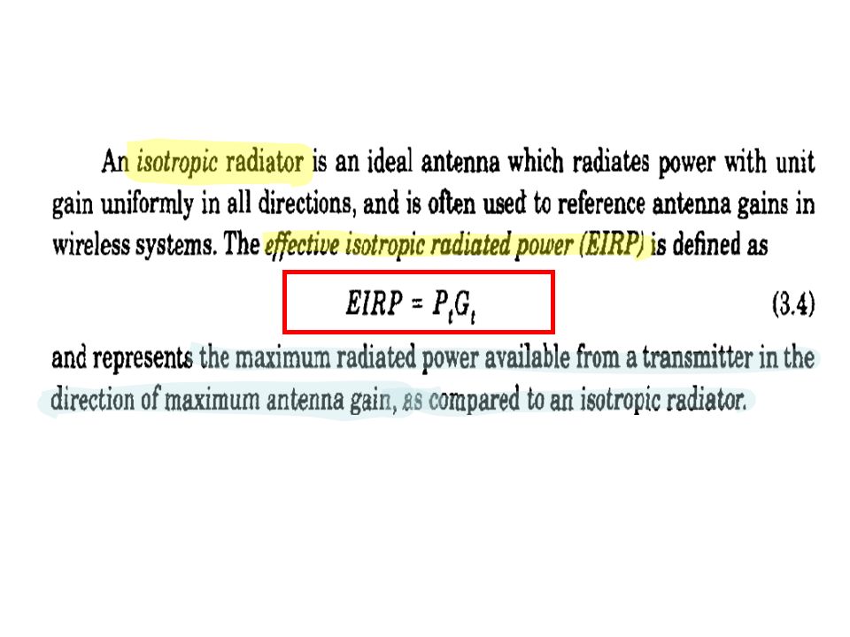
19. In practice, effective radiated power (ERP) is used instead of EIRP to denote the maximum radiated power as compared to a half-wave dipole antenna (instead of an isotropic antenna). Since a dipole antenna has a gain of 1.64 (2.15 dB above an isotropic), the ERP will be 2.15 dB smaller than the EIRP for the same transmission system. In practice, antenna gains are given in units of dBi (dB gain with respect to an isotropic source) or dBd (dB gain with respect to a half-wave dipole)

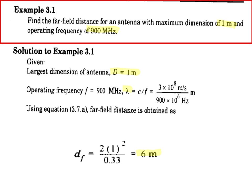
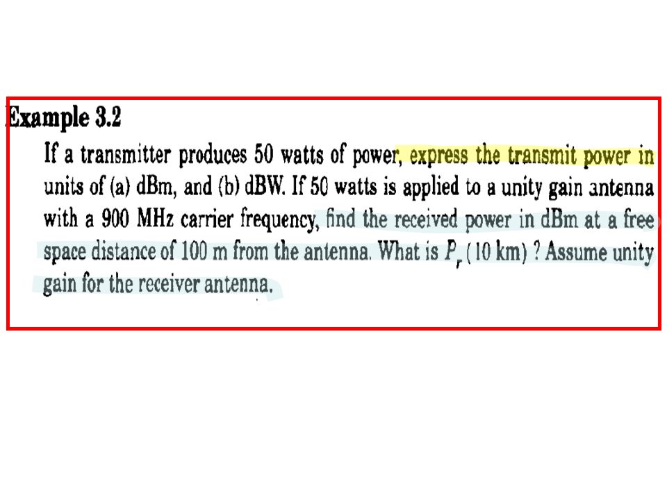
23. a close-in distance, d0, as a known received power reference point. The received power, P r (d). at any distance d > d 0, The reference distance must be chosen such that it lies in the far-field region, that is, d 0 > d f, and d 0 is chosen to be smaller than any practical distance used in the mobile communication system. may be expressed in units of dBm or dBW by simply taking the logarithm of both sides and multiplying by 10. For example, if Pr is in units of dBm, the received power is given by