1. Market Equilibrium Week 3

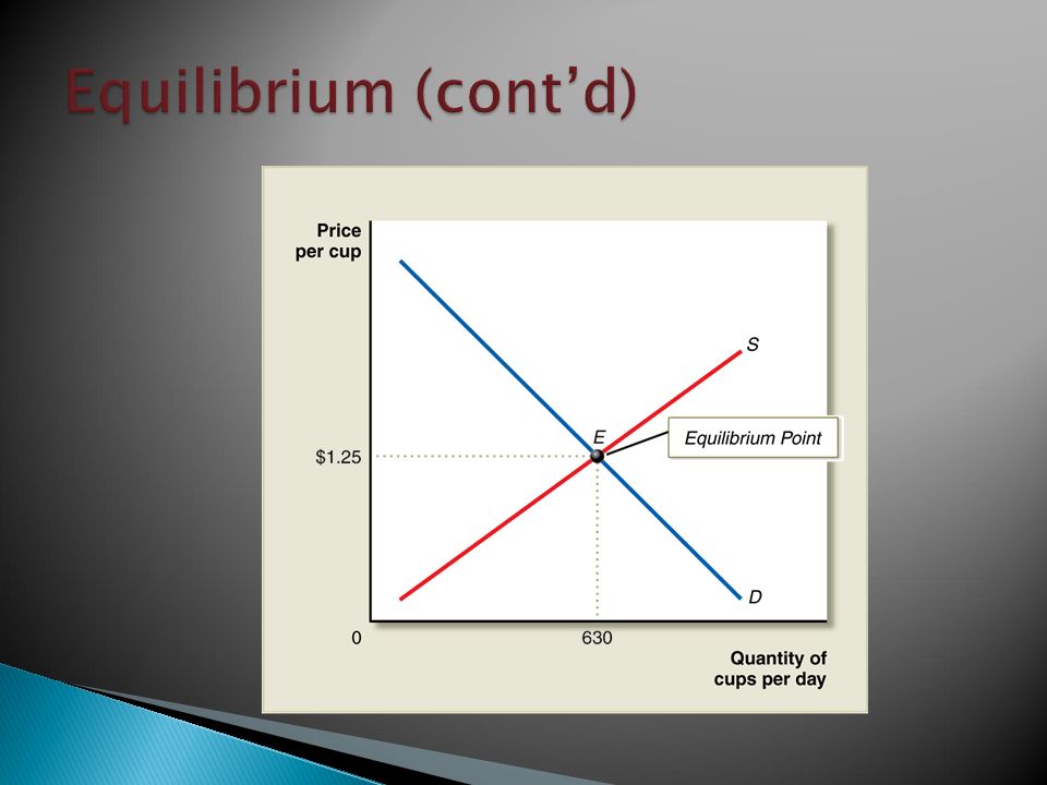
3.  At the market equilibrium price: ◦ Quantity demanded by consumers = quantity supplied by firms/producers/sellers ◦ Without a change in any of the ceterius paribus conditions, the price will remain unchanged

4.  Consumers ◦ Willing to buy another unit, if market price <= to marginal (use) value of consuming it  Suppliers ◦ Willing to sell/produce another unit, if market price >= marginal (additional) costs of producing the last unit  Equilibrium occurs only when ◦ MV consumer = P market = MC producer

5.  MV MC ◦ Sellers are willing to continue to supply more goods ◦ Consumers are unwilling to buy ◦ Excess supply will lead to sellers dropping their prices down in the future to clear inventory  MV > P < MC ◦ Sellers not willing to supply as much as consumers will demand (excess demand) ◦ Excess demand will lead to consumers bidding prices up to get the “shortage”

6.  At each price, determine whether there would be a shortage (Qd > Qs) or a surplus (Qs > Qd)  If there was a shortage, how would price adjust to clear the market?  If there is a surplus, how would price adjust to clear the market? # of Pizzas Demand ed Price Per Pizza # of Pizzas Supplie d Shortage or Surplus 1000$10400 900$12450 800$14500 700$16550 600$18600 500$20650

7.  http://www.bized.co.uk/current/mind/2004_5/251004. ppt http://www.bized.co.uk/current/mind/2004_5/251004. ppt  Hungarian-born economist Nicholas Kaldor (1908- 1986)Nicholas Kaldor  Simple dynamic model of cyclical demand with time lags between the response of production and a change in price (most often seen in agricultural sectors).  Cobweb theory is the process of adjustment in markets  Traces the path of prices and outputs in different equilibrium situations. Path resembles a cobweb with the equilibrium point at the center of the cobweb.  Sometimes referred to as the hog-cycle (after the phenomenon observed in American pig prices during the 1930s).

8. D S 7 Price (£) Quantity Bought and Sold (millions) 9 D1 In a ‘divergent cobweb’ - also termed an unstable cobweb - the price tends to move away from equilibrium. Assume the initial equilibrium price is £7 and the quantity 9. If demand rises, the shortage pushes the price up to £11 per turkey. 11 15 Farmers respond by planning to increase supply, ten months later, the supply of turkeys is 15 million. At this level, there will be a surplus of turkeys and the price drops. 8 The price falls to £5 and farmers react by cutting plans for turkey production. Ten months later, supply on the market will be 8 million. 5 This creates a massive shortage of 9 million turkeys and the price is forced up – and so the process continues! A divergent cobweb leads to price instability over time. 17

9.  Consumer surplus ◦ Difference between what you are willing-to-pay and what you have to pay  Willingness-to-pay ◦ Everything under the demand curve up to the last unit that you bought  What you had to pay ◦ Average price paid x number of units purchased

10. Demand Curve is Also Marginal Value and Avg Revenue Amount Paid CS Total WTP = CS + Amt Paid

11.  Producer Surplus ◦ The difference between what they get paid (total revenues) and what it costs them  Total Revenues ◦ > = Average Price x Quantity Purchased  Total Costs ◦ > = Sum of Marginal Costs up to the amount supplied (Q S )  Or = the area under the supply curve up to Q s

12.  Value of the market  To Consumers = Consumer Surplus  To Producers = Producer Surplus  Value equals the sum of both CS and PS

13.  Evaluating the market equilibrium  Market outcomes 1.Free markets allocate the supply of goods to the buyers who value them most highly  Measured by their willingness to pay 2.Free markets allocate the demand for goods to the sellers who can produce them at the least cost  Only produce if you are paid as much (or more) than product costs to make (MC) 13

14. 7 14 Price Total surplus—the sum of consumer and producer surplus—is the area between the supply and demand curves up to the equilibrium quantity 0 Quantity Equilibrium quantity Equilibrium price Demand Supply Consumer surplus Producer surplus B C A D E

15.  Evaluating the market equilibrium ◦ Social planner  Cannot increase economic well-being by  Changing the allocation of consumption among buyers  Changing the allocation of production among sellers  Cannot rise total economic well-being by  Increasing or decreasing the quantity of the good 3.Free markets produce the quantity of goods that maximizes the sum of consumer and producer surplus 15

16. 8 16 Price At quantities less than the equilibrium quantity, such as Q 1, the value to buyers exceeds the cost to sellers. At quantities greater than the equilibrium quantity, such as Q 2, the cost to sellers exceeds the value to buyers. Therefore, the market equilibrium maximizes the sum of producer and consumer surplus. 0 Quantity Equilibrium quantity Demand Supply Q1Q1 Q2Q2 Value to buyers Value to buyers Cost to sellers Cost to sellers Value to buyers is greater than cost to sellers Value to buyers is less than cost to sellers

17.  Evaluating the market equilibrium  Equilibrium outcome ◦ Efficient allocation of resources ◦ Consumers:  Goods to those who value it most (MV >= P) ◦ Suppliers  Goods produced by those with least costs/most efficient production (P>MC) ◦ Efficient use of resources  Produce only goods whose value is >= cost of using the resources 17

18.  In the world ◦ Competition - far from perfect  Market power  A single buyer or seller (small group)  Control market prices  Markets are inefficient  Keeps the price and quantity away from the equilibrium of supply and demand 18

19.  In the world ◦ Decisions of buyers and sellers  Affect people who are not participants in the market at all  Externalities  Cause welfare in a market to depend on more than just the value to the buyers and the cost to the sellers  Inefficient equilibrium  From the standpoint of society as a whole 19

20.  Market failure ◦ E.g.: market power and externalities ◦ The inability of some unregulated markets to allocate resources efficiently ◦ Occurs only in specific market types:  Monopoly  Possibly oligopoly (small number of producers)  Externalities (pollution, fish, natural resources)  Asymmetric information (financial markets) ◦ Public policy  Can potentially remedy the problem  Increase economic efficiency 20