1. Designing Parallel Programs  Automatic vs. Manual Parallelization  Understand the Problem and the Program  Communications  Synchronization  Data Dependencies

2. Designing Parallel Programs  Load Balancing  Granularity  I/O  Limits and Costs of Parallel Programming  Performance Analysis and Tuning

3. Automatic vs. Manual Parallelization Designing and developing parallel programs has characteristically been a very manual process. The programmer is typically responsible for both identifying and actually implementing parallelism. Very often, manually developing parallel codes is a time consuming, complex, error-prone and iterative process.

4. Automatic vs. Manual Parallelization For a number of years now, various tools have been available to assist the programmer with converting serial programs into parallel programs. The most common type of tool used to automatically parallelize a serial program is a parallelizing compiler or pre-processor.

5. Automatic vs. Manual Parallelization A parallelizing compiler generally works in two different ways: – Fully Automatic The compiler analyzes the source code and identifies opportunities for parallelism.

6. Automatic vs. Manual Parallelization The analysis includes identifying inhibitors to parallelism and possibly a cost weighting on whether or not the parallelism would actually improve performance. Loops (do, for) loops are the most frequent target for automatic parallelization.

7. Automatic vs. Manual Parallelization – Programmer Directed Using "compiler directives" or possibly compiler flags, the programmer explicitly tells the compiler how to parallelize the code. May be able to be used in conjunction with some degree of automatic parallelization also.

8. Automatic vs. Manual Parallelization If you are beginning with an existing serial code and have time or budget constraints, then automatic parallelization may be the answer.

9. Automatic vs. Manual Parallelization However, there are several important caveats that apply to automatic parallelization: – Wrong results may be produced – Performance may actually degrade – Much less flexible than manual parallelization

10. Automatic vs. Manual Parallelization – Limited to a subset (mostly loops) of code – May actually not parallelize code if the analysis suggests there are inhibitors or the code is too complex Parallel algorithms for MIMD machines discussed earlier applies to the manual method of developing parallel codes.

11. recap  Pipelined Algorithms / Algorithmic Parallelism  Partitioned Algorithms / Geometric Parallelism  Asynchronous / Relaxed Algorithms

12. Understand the Problem and the Program  Undoubtedly, the first step in developing parallel software is to first understand the problem that you wish to solve in parallel.  If you are starting with a serial program, this necessitates understanding the existing code also.  Before spending time in an attempt to develop a parallel solution for a problem,  determine whether or not the problem is one that can actually be parallelized.

13. Example of Parallelizable Problem:  Calculate the potential energy for each of several thousand independent conformations of a molecule.  When done, find the minimum energy conformation.  This problem is able to be solved in parallel.  Each of the molecular conformations is independently determinable.  The calculation of the minimum energy conformation is also a parallelizable problem.

14. Example of a Non-parallelizable Problem:  Calculation of the Fibonacci series (0,1,1,2,3,5,8,13,21,...) by use of the formula:  F(n) = F(n-1) + F(n-2)  This is a non-parallelizable problem because the calculation of the Fibonacci sequence as shown would entail dependent calculations rather than independent ones.

15. Example of a Non-parallelizable Problem  The calculation of the F(n) value uses those of both F(n-1) and F(n-2).  These three terms cannot be calculated independently and therefore, not in parallel.

16. Understand the Problem and the Program  Identify the program's hotspots:  Know where most of the real work is being done. The majority of scientific and technical programs usually accomplish most of their work in a few places.  Profilers and performance analysis tools can help here  Focus on parallelizing the hotspots and ignore those sections of the program that account for little CPU usage.

17. Understand the Problem and the Program  Identify bottlenecks in the program  Are there areas that are disproportionately slow, or cause parallelizable work to halt or be deferred? For example, I/O is usually something that slows a program down.  May be possible to restructure the program or use a different algorithm to reduce or eliminate unnecessary slow areas

18. Understand the Problem and the Program  Identify inhibitors to parallelism. One common class of inhibitor is data dependence, as demonstrated by the Fibonacci sequence above.  Investigate other algorithms if possible.  This may be the single most important consideration when designing a parallel application.

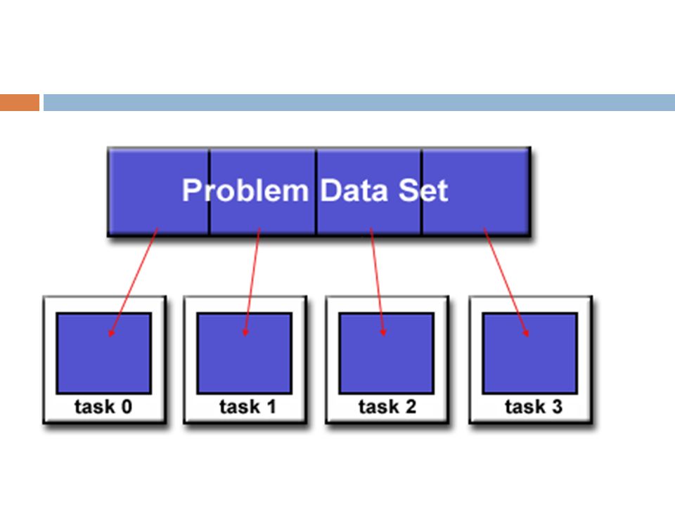
19. Partitioning  One of the first steps in designing a parallel program is to break the problem into discrete "chunks" of work that can be distributed to multiple tasks.  This is known as decomposition or partitioning.  There are two basic ways to partition computational work among parallel tasks:  domain decomposition and functional decomposition

20. Domain Decomposition:  In this type of partitioning, the data associated with a problem is decomposed.  Each parallel task then works on a portion of the data.

22.  There are different ways to partition data:

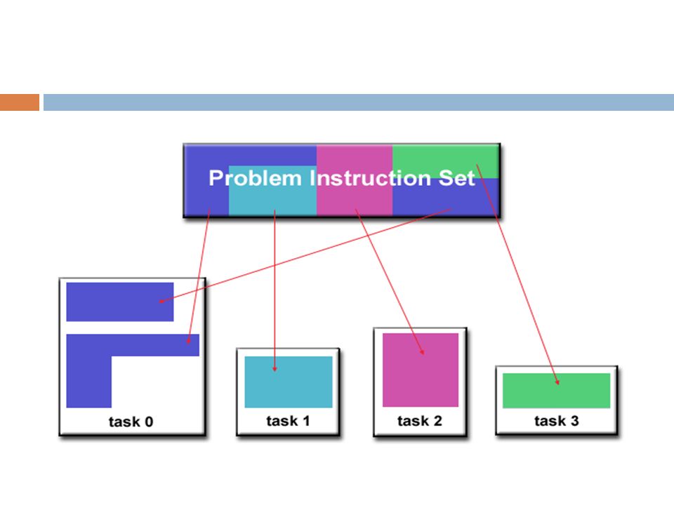
23. Functional Decomposition:  In this approach, the focus is on the computation that is to be performed rather than on the data manipulated by the computation.  The problem is decomposed according to the work that must be done.  Each task then performs a portion of the overall work.

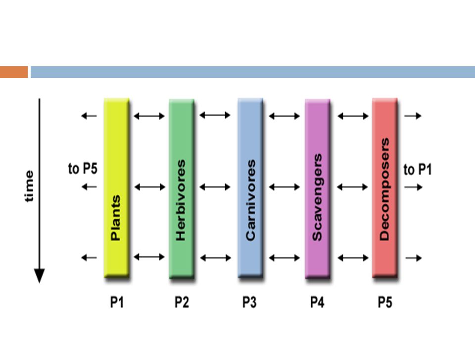
25.  Functional decomposition lends itself well to problems that can be split into different tasks.  For example:  Ecosystem Modeling Each program calculates the population of a given group, where each group's growth depends on that of its neighbors.

26.  As time progresses, each process calculates its current state, then exchanges information with the neighbor populations.  All tasks then progress to calculate the state at the next time step.

28. Communications  The need for communications between tasks depends upon your problem:  You DON'T need communications  Some types of problems can be decomposed and executed in parallel with virtually no need for tasks to share data.  For example, imagine an image processing operation where every pixel in a black and white image needs to have its color reversed.  The image data can easily be distributed to multiple tasks that then act independently of each other to do their portion of the work.  These types of problems are often called embarrassingly parallel because they are so straight-forward.  Very little inter-task communication is required.

29.  You DO need communications  Most parallel applications are not quite so simple, and do require tasks to share data with each other.  For example, a 3-D heat diffusion problem requires a task to know the temperatures calculated by the tasks that have neighboring data.  Changes to neighboring data has a direct effect on that task's data.

30. Factors to Consider  Cost of communications  Inter-task communication virtually always implies overhead.  Machine cycles and resources that could be used for computation are instead used to package and transmit data.  Communications frequently require some type of synchronization between tasks, which can result in tasks spending time "waiting" instead of doing work.  Competing communication traffic can saturate the available network bandwidth, further aggravating performance problems.

31. Factors to Consider  Latency vs. Bandwidth  latency is the time it takes to send a minimal (0 byte) message from point A to point B.  Commonly expressed as microseconds.  bandwidth is the amount of data that can be communicated per unit of time.

32. Factors to Consider  Commonly expressed as megabytes/sec or gigabytes/sec.  Sending many small messages can cause latency to dominate communication overheads.  Often it is more efficient to package small messages into a larger message, thus increasing the effective communications bandwidth.

33. Factors to Consider  Visibility of communications  With the Message Passing Model,  communications are explicit and generally quite visible and under the control of the programmer.

34. Factors to Consider  With the Data Parallel Model,  communications often occur transparently to the programmer, particularly on distributed memory architectures.  The programmer may not even be able to know exactly how inter-task communications are being accomplished.

35. Synchronous vs. asynchronous communications  Synchronous communications require some type of "handshaking" between tasks that are sharing data.  This can be explicitly structured in code by the programmer, or it may happen at a lower level unknown to the programmer.  Synchronous communications are often referred to as blocking communications since other work must wait until the communications have completed.

36. Synchronous vs. asynchronous communications  Asynchronous communications allow tasks to transfer data independently from one another.  For example, task 1 can prepare and send a message to task 2, and then immediately begin doing other work.  When task 2 actually receives the data doesn't matter.

37. Synchronous vs. asynchronous communications  Asynchronous communications are often referred to as non-blocking communications since  other work can be done while the communications are taking place.  Interleaving computation with communication is the single greatest benefit for using asynchronous communications.

38. Scope of communications  Knowing which tasks must communicate with each other is critical during the design stage of a parallel code.  Both of the two scopings described below can be implemented synchronously or asynchronously.

39. Scope of communications  Point-to-point - involves two tasks with one task acting as the sender/producer of data, and the other acting as the receiver/consumer.  Collective - involves data sharing between more than two tasks, which are often specified as being members in a common group, or collective.

40. Efficiency of communications  Very often, the programmer will have a choice with regard to factors that can affect communications performance.  Which implementation for a given model should be used?  Using the Message Passing Model as an example,

41. Efficiency of communications  one MPI implementation may be faster on a given hardware platform than another.  What type of communication operations should be used?  As mentioned previously, asynchronous communication operations can improve overall program performance.

42. Efficiency of communications  Network media - some platforms may offer more than one network for communications.  Which one is best?

43. Synchronization  Types of Synchronization:  Barrier  Usually implies that all tasks are involved  Each task performs its work until it reaches the barrier.  It then stops, or "blocks".

44. Barrier  When the last task reaches the barrier, all tasks are synchronized.  What happens from here varies.  Often, a serial section of work must be done.  In other cases, the tasks are automatically released to continue their work.

45. Lock / semaphore  Can involve any number of tasks  Typically used to serialize (protect) access to global data or a section of code.  Only one task at a time may use (own) the lock / semaphore / flag.

46. Lock / semaphore  The first task to acquire the lock "sets" it.  This task can then safely (serially) access the protected data or code.  Other tasks can attempt to acquire the lock but must wait until the task that owns the lock releases it.  Can be blocking or non-blocking

47. Synchronous communication operations  Involves only those tasks executing a communication operation  When a task performs a communication operation,  some form of coordination is required with the other task(s) participating in the communication.  For example, before a task can perform a send operation,  it must first receive an acknowledgment from the receiving task that it is OK to send.

48. Data Dependencies  Definition:  A dependence exists between program statements when the order of statement execution affects the results of the program.  A data dependence results from multiple use of the same location(s) in storage by different tasks.  Dependencies are important to parallel programming because they are one of the primary inhibitors to parallelism.

49. Examples:  Loop carried data dependence  DO 500 J = MYSTART,MYEND A(J) = A(J-1) * 2.0  500 CONTINUE  The value of A(J-1) must be computed before the value of A(J),  therefore A(J) exhibits a data dependency on A(J-1). Parallelism is inhibited.

50. Data Dependencies  If Task 2 has A(J) and task 1 has A(J-1), computing the correct value of A(J) necessitates:  Distributed memory architecture - task 2 must obtain the value of A(J-1) from task 1 after task 1 finishes its computation  Shared memory architecture - task 2 must read A(J-1) after task 1 updates it

51. Data Dependencies  Loop independent data dependence   task 1 task 2  ------ ------   X = 2 X = 4 ..  Y = X**2 Y = X**3

52. Data Dependencies  As with the previous example, parallelism is inhibited. The value of Y is dependent on:  Distributed memory architecture - if or when the value of X is communicated between the tasks.  Shared memory architecture - which task last stores the value of X.

53. Data Dependencies  Although all data dependencies are important to identify when designing parallel programs,  loop carried dependencies are particularly important  since loops are possibly the most common target of parallelization efforts.

54. Data Dependencies  How to Handle Data Dependencies:  Distributed memory architectures - communicate required data at synchronization points.  Shared memory architectures -synchronize read/write operations between tasks.

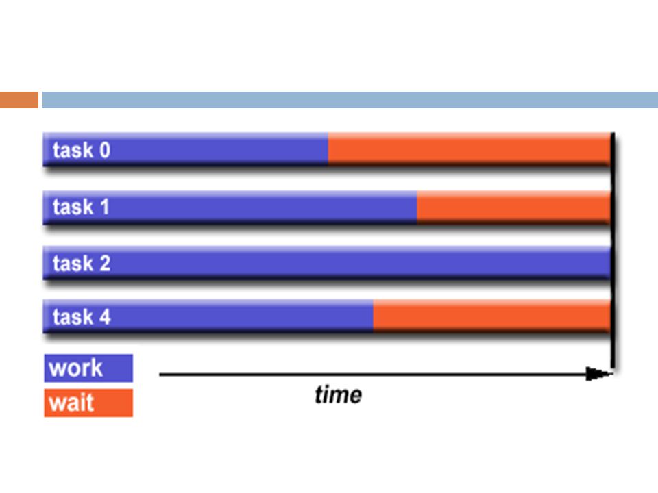
55. Load Balancing  Load balancing refers to the practice of distributing work among tasks so that all tasks are kept busy all of the time.  It can be considered a minimization of task idle time.  Load balancing is important to parallel programs for performance reasons.  For example, if all tasks are subject to a barrier synchronization point, the slowest task will determine the overall performance.

57. How to Achieve Load Balance:  Equally partition the work each task receives  For array/matrix operations where each task performs similar work,  evenly distribute the data set among the tasks.  For loop iterations where the work done in each iteration is similar, evenly distribute the iterations across the tasks.

58.  If a heterogeneous mix of machines with varying performance characteristics are being used,  be sure to use some type of performance analysis tool to detect any load imbalances.  Adjust work accordingly.

59.  Use dynamic work assignment  Certain classes of problems result in load imbalances even if data is evenly distributed among tasks:

60.  Sparse arrays - some tasks will have actual data to work on while others have mostly "zeros".  Adaptive grid methods - some tasks may need to refine their mesh while others don't.  N-body simulations - where some particles may migrate to/from their original task domain to another task's; where the particles owned by some tasks require more work than those owned by other tasks.

61.  When the amount of work each task will perform is intentionally variable, or is unable to be predicted, it may be helpful to use a scheduler - task pool approach. As each task finishes its work, it queues to get a new piece of work.  It may become necessary to design an algorithm which detects and handles load imbalances as they occur dynamically within the code.

62. Granularity  Computation / Communication Ratio:  In parallel computing, granularity is a qualitative measure of the ratio of computation to communication.  Periods of computation are typically separated from periods of communication by synchronization events.

63. Fine-grain Parallelism:  Relatively small amounts of computational work are done between communication events  Low computation to communication ratio  Facilitates load balancing

64.  Implies high communication overhead and less opportunity for performance enhancement  If granularity is too fine it is possible that the overhead required for communications and synchronization between tasks takes longer than the computation.

65. Coarse-grain Parallelism:  Relatively large amounts of computational work are done between communication/synchronization events  High computation to communication ratio  Implies more opportunity for performance increase  Harder to load balance efficiently

66. Which is Best?  The most efficient granularity is dependent on the algorithm and the hardware environment in which it runs.  In most cases the overhead associated with communications and synchronization is high relative to execution speed so it is advantageous to have coarse granularity.  Fine-grain parallelism can help reduce overheads due to load imbalance.

67. I/O  The Bad News:  I/O operations are generally regarded as inhibitors to parallelism  Parallel I/O systems may be immature or not available for all platforms

68.  In an environment where all tasks see the same file space, write operations can result in file overwriting  Read operations can be affected by the file server's ability to handle multiple read requests at the same time  I/O that must be conducted over the network (NFS, non-local) can cause severe bottlenecks and even crash file servers.

69. I/O  The Good News:  Parallel file systems are available. For example:  GPFS: General Parallel File System for AIX (IBM)  Lustre: for Linux clusters (Oracle)  The parallel I/O programming interface specification for MPI has been available since 1996 as part of MPI-2. Vendor and "free" implementations are now commonly available.

70. A few pointers:  Rule #1: Reduce overall I/O as much as possible  If you have access to a parallel file system, investigate using it.  Writing large chunks of data rather than small packets is usually significantly more efficient.

71.  Confine I/O to specific serial portions of the job, and then use parallel communications to distribute data to parallel tasks.  For example, Task 1 could read an input file and then communicate required data to other tasks.  Likewise, Task 1 could perform write operation after receiving required data from all other tasks.

72.  Use local, on-node file space for I/O if possible.  For example, each node may have /tmp filespace which can used.  This is usually much more efficient than performing I/O over the network to one's home directory.

73. Limits and Costs of Parallel Programming  Amdahl's Law:  Amdahl's Law states that potential program speedup is defined by the fraction of code (P) that can be parallelized:  speedup = 1/(1 - P )

74.  If none of the code can be parallelized, P = 0 and the speedup = 1 (no speedup).  If all of the code is parallelized, P = 1 and the speedup is infinite (in theory).  If 50% of the code can be parallelized, maximum speedup = 2, meaning the code will run twice as fast.

75.  Introducing the number of processors performing the parallel fraction of work, the relationship can be modeled by:  speedup = 1(P/N + S)  where P = parallel fraction, N = number of processors and S = serial fraction.

76.  It soon becomes obvious that there are limits to the scalability of parallelism. For example: speedup -------------------------------- N P =.50 P =.90 P =.99 ----- ------- ------- ------- 10 1.82 5.26 9.17 100 1.98 9.17 50.25 1000 1.99 9.91 90.99 10000 1.99 9.91 99.02 100000 1.99 9.99 99.90

77.  However, certain problems demonstrate increased performance by increasing the problem size.  For example:  2D Grid Calculations 85 seconds 85%  Serial fraction 15 seconds 15%

78.  We can increase the problem size by doubling the grid dimensions and halving the time step.  This results in four times the number of grid points and twice the number of time steps.  The timings then look like:  2D Grid Calculations 680 seconds 97.84%  Serial fraction 15 seconds 2.16%

79.  Problems that increase the percentage of parallel time with their size are more scalable than problems with a fixed percentage of parallel time.

80. Complexity:  In general, parallel applications are much more complex than corresponding serial applications, perhaps an order of magnitude.  Not only do you have multiple instruction streams executing at the same time, but you also have data flowing between them.

81.  The costs of complexity are measured in programmer time in virtually every aspect of the software development cycle:  Design  Coding  Debugging  Tuning  Maintenance

82.  Adhering to "good" software development practices is essential when working with parallel applications –  especially if somebody besides you will have to work with the software.

83. Portability  Thanks to standardization in several APIs, such as MPI, POSIX threads, HPF and OpenMP, portability issues with parallel programs are not as serious as in years past.  However...  All of the usual portability issues associated with serial programs apply to parallel programs.

84.  For example, if you use vendor "enhancements" to Fortran, C or C++, portability will be a problem.  Even though standards exist for several APIs, implementations will differ in a number of details, sometimes to the point of requiring code modifications in order to effect portability.

85.  Operating systems can play a key role in code portability issues.  Hardware architectures are characteristically highly variable and can affect portability.

86. Resource Requirements:  The primary intent of parallel programming is to decrease execution wall clock time, however in order to accomplish this, more CPU time is required.  For example, a parallel code that runs in 1 hour on 8 processors actually uses 8 hours of CPU time.

87.  The amount of memory required can be greater for parallel codes than serial codes, due to the need to replicate data and for overheads associated with parallel support libraries and subsystems.  For short running parallel programs, there can actually be a decrease in performance compared to a similar serial implementation.

88.  The overhead costs associated with setting up the parallel environment, task creation, communications and task termination can comprise a significant portion of the total execution time for short runs.

89. Scalability:  The ability of a parallel program's performance to scale is a result of a number of interrelated factors.  Simply adding more machines is rarely the answer.  The algorithm may have inherent limits to scalability.

90.  At some point, adding more resources causes performance to decrease.  Most parallel solutions demonstrate this characteristic at some point.  Hardware factors play a significant role in scalability.

91.  Examples:  Memory-cpu bus bandwidth on an SMP machine  Communications network bandwidth  Amount of memory available on any given machine or set of machines  Processor clock speed  Parallel support libraries and subsystems software can limit scalability independent of your application