2. Outline  Introduction  Subgraph Pattern Matching  Types of Subgraph Pattern Matching  Models of Computation  Distributed Algorithms  Performance Evaluation  Graph Partitioning  Results Analysis  Conclusion

3. Introduction  Directed graph G(V, E, l)  V is a set of vertices  E ⊆ V x V is a set of directed edges  l: V → is a function mapping vertices to labels  Versatility and expressivity  Social networks, web search engines, genome sequencing, etc.  Data sizes are growing rapidly  Facebook: 1 billion + users, average degree of 140  Twitter: 200 million + users, 400 million tweets each day  Bigger datasets mean bigger graphs

4. Subgraph Pattern MatchingSubgraph Pattern Matching  A graph G’(V’, E’, l’) is a subgraph of G(V, E, l) if: 1.V’ ⊆ V 2. E’ ⊆ V’ x V’ ⊆ E 3. ∀ v ∈ V’, l’(v) = l(v)  A pattern (or query ) is a graph that we want to find in a bigger graph  Subgraph pattern matching: Given a query graph, find all subgraphs of another graph (the data graph) that are similar to the query based on certain criteria

5. Types of Subgraph Pattern Matching  Exact  Subgraph Isomorphism  Heuristic  Graph Simulation  Dual Simulation  Strong Simulation

6. Subgraph IsomorphismSubgraph Isomorphism  Exact matching from the pattern to data graph  Labels must be the same  Ullmann’s algorithm, VF2  NP-hard problem in general case  Current solutions not practical for large graphs

7. Example: Subgraph Isomorphism Matches: {4, 8, 6, 7}, {5, 8, 6, 7}

8. Graph SimulationGraph Simulation  A vertex in a data graph G matches a vertex in query graph Q via graph simulation iff 1.both have the same label 2.a subset of its children match all the children of its corresponding vertex in the query graph  HHK algorithm [1] [1] M. R. Henzinger, T. A. Henzinger, and P. W. Kopke, “Computing simulations on finite and infinite graphs,” in Foundations of Computer Science, 1995. Proceedings., 36th Annual Symposium on. IEEE, 1995, pp. 453–462.

9. Graph SimulationGraph Simulation

10. Dual SimulationDual Simulation  Adds a duality condition to graph simulation  A vertex in a data graph becomes a match with a vertex in the query graph iff 1.Both have the same label 2.A subset of its children matches all the children of its corresponding vertex in the data graph 3.A subset of its parents matches all the parents of its corresponding vertex in the data graph  O((| V q | + | E q |) (| V | + | E |))  More restrictive than graph simulation

11. Example: Graph  Dual Simulation

13. Strong SimulationStrong Simulation  Extends dual simulation with a locality condition  A ball G [ v, r ] is a subset of a graph G containing:  all vertices V B within an undirected distance r of the vertex v  all the edges between the vertices in V B

14. Strong SimulationStrong Simulation  Extends dual simulation with a locality condition  A ball G [ v, r ] is a subset of a graph G containing:  all vertices V B within an undirected distance r of the vertex v  all the edges between the vertices in V B

15. Strong SimulationStrong Simulation  Extends dual simulation with a locality condition  A ball G [ v, r ] is a subset of a graph G containing:  all vertices V B within an undirected distance r of the vertex v  all the edges between the vertices in V B  O( |V |(| V | + (| V q | + | E q |) (| V | + | E |))  Query graph Q(V q, E q, l) matches data graph G(V, E, l) via strong simulation if there exists a vertex v ∈ V s.t. 1. Q matches G [ v, d q ] via dual simulation with match relation R b 2. v is contained in R b

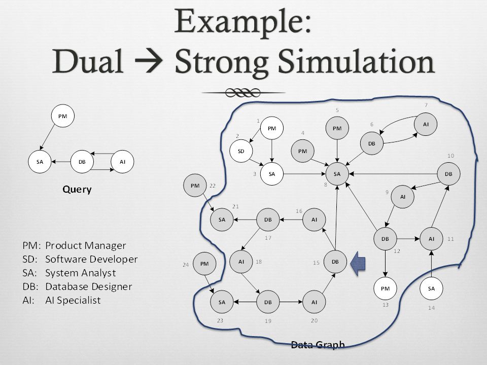
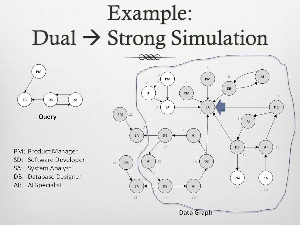
16. Example: Dual  Strong Simulation

20. Models of ComputationModels of Computation MapReduce Useful paradigm for large batch processing of datasets Not ideal for many graph algorithms Bulk Synchronous Parallel (BSP) Computation performed in a series of supersteps Interleaved with communication/synchronization phases Vertex-Centric (VC) BSP Each vertex treated as a processing unit Vertices can communicate with each other to obtain information Message Passing Different threads communicate with each other via messages Programmer has more control over communication and synchronization

21. Distributed Graph SimulationDistributed Graph Simulation Superstep 1:If there is any query vertex with the same label: - Set match to true - Make a match set of potential vertices in the query - Ask children about their status Otherwise: Vote to halt Superstep 2:If match is true : Reply back to parent with label Otherwise: Vote to halt Superstep 3:If match is true : - Evaluate match set based on children’s responses - If there are removals from the match set: - Inform parents - Set match flag accordingly - Otherwise: Vote to halt Otherwise: Vote to halt Superstep 4:If there is any incoming removal message: - Evaluate match set based on children’s responses - If there are removals from the match set: - Inform parents - Set match flag accordingly - Otherwise: Vote to halt Otherwise: Vote to halt

22. Distributed Graph SimulationDistributed Graph Simulation

23. Other Distributed Graph Algorithms  Dual simulation  Similar to graph simulation  In addition to storing the match sets of its children, a vertex also stores the match sets of its parents  During match set evaluation, a vertex takes both of these into account  Strong simulation (optimized)  First run dual simulation to obtain match relation R  For each matching vertex v in R :  Create a ball centered at v with radius d q containing only vertices in R  Perform dual simulation on the ball

24. Performance EvaluationPerformance Evaluation  Experimental setup  Cluster with 12 machines  Each with two 2Ghz Intel Xeon E5-2620 CPUs, each with six cores  Ethernet: 1 Gb/s  Set up HDFS/GPS on all of the machines Dataset|V||E| | l| Synthesized100 M4 B200 uk-200539 M940 M200 enwiki-20054.2 M101 M200

25. Runtime EvaluationRuntime Evaluation Synthesized, |V|= 10 8

26. Runtime EvaluationRuntime Evaluation uk-2005, |V|= 3.9 x 10 7

27. Runtime EvaluationRuntime Evaluation enwiki-2013, |V|= 4.2 x 10 6

28. Speedup EvaluationSpeedup Evaluation Synthesized, |V|= 10 8

29. Speedup EvaluationSpeedup Evaluation uk-2005, |V|= 3.9 x 10 7

30. Speedup EvaluationSpeedup Evaluation enwiki-2013, |V|= 4.2 x 10 6

31. Conclusions  The three algorithms exhibit excellent scalable behavior in terms of speedup and efficiency as we increase the number of workers  Distributed implementations (GPS):  Graph simulation  Dual simulation  Strong simulation  Ongoing work:  Distributed implementations with message passing in Akka  Our own sequential/distributed isomorphism algorithm

32. Questions?

33. Thanks

34. Depth-First BallDepth-First Ball  Algorithm works in a depth-first fashion. Message is generated at the center which is then propagated through the system for ballSize supersteps.  The approach results in an exponential number of messages that slows down the whole system and renders the approach impractical

35. Breadth-First BallBreadth-First Ball  Works on a simple ping-reply model.  Center vertex starts of by sending a ping message to all of its adjacent nodes in the first superstep.  In the second superstep, all the recipient nodes reply back with their label and the ids of their children and parents.  Center vertex upon receiving this information in the third superstep, saves the returned labels and then ping the boundary nodes. This process is repeated till we have a ball of size d q.

36. Breadth-First BallBreadth-First Ball

37. Efficiency Synthesized, |V|=10 8 uk-2005, |V|=3.9x10 7 enwiki-2013, |V|=4.2x10 6 Calculated as Efficiency k = Speedup k /k

38. Graph PartitioningGraph Partitioning  By default, the data graph is partitioned in a round-robin fashion among workers  The goals of min-cut partitioning are two-fold:  to create well-balanced partitions  to reduce the inter-partition edges  Number of other algorithms have been shown to use min-cut graph partitioning successfully for speed-ups  METIS 1 – graph partitioning tool  Written in C  Takes an undirected graph and outputs the partitions 1 http://glaros.dtc.umn.edu/gkhome/metis/m etis/overview

39. Performance EvaluationPerformance Evaluation  Experimental Setup  Cluster with 5 machines  Each with two 2Ghz Intel Xeon E5-2620 CPU, each with six cores  Ethernet: 1 Gb/sec  Setup HDFS/GPS on all the machines  Datasets:  Labels ( l ) = 200 Datasets|V||E| Synthesized10 7 251 x 10 6 uk-20021.8 x 10 7 298 x 10 6

40. Results - RuntimeResults - Runtime Graph Simulation Dual Simulation Strict Simulation

41. Results - RuntimeResults - Runtime uk-2002, |V|=1.8x10 7 Graph Simulation Dual Simulation Strict Simulation

42. Results – Network I/OResults – Network I/O Graph Simulation Dual Simulation Strict Simulation

43. Results – Network I/OResults – Network I/O uk-2002, |V|=1.8x10 7 Graph Simulation Dual Simulation Strict Simulation

44. Planned Pattern Matching Implementations SequentialDistributed (GPS) Distributed (Akka VC) Distributed (Akka MP) Graph Simulation 0.581 s2.924 s---------- Dual Simulation 0.642 s3.403 s---------- Strong Simulation ----------8.453 s---------- Subgraph Iso. (ours) 2.837 s---------- Subgraph Iso. (VF2) ----------