Download presentation
Presentation is loading. Please wait.

1
Pipe flow analysis

2
Pipe flow & Open channel flow
The pipe is assumed to be completely full of the flowing fluid. Driving force for open channel is only gravity Pipe flow is driven by pressure difference & gravity( if not horizontal)
")
3
Laminar and Turbulent Flow
For laminar flow in a pipe there is only one component For turbulent flow the predominant component of velocity is also along the pipe, but it is unsteady (random) and accompanied by random components normal to the pipe axis,
 and accompanied by random components normal to the pipe axis,")
4
Pipe flow characteristics are dependent on the value of the Reynolds number

5
Hegen’s experimental result

6
Entrance Region and Fully Developed Flow

8
The entrance length is a function of the Reynolds number

10
Continuity equation Energy equation Momentum equation

12
Finding out f for laminar & turbulent flow
Steady, fully developed pipe flow experiences no acceleration. 1

13
2 Basic pipe flow is governed by a balance between viscous and pressure forces. From 1 & 2 3

14
How the shear stress is related to the velocity?
This is the critical step that separates the analysis of laminar from that of turbulent flow Newton’s law of motion Laminar flow of Newtonian fluid

15
Where Where

16
For non horizontal pipe
For a laminar flow(Re<2100) in a horizontal pipe the flowrate is (a) directly proportional to the pressure drop, (b) inversely proportional to the viscosity, (c) inversely proportional to the pipe length, and (d) proportional to the pipe diameter to the fourth power. This flow, the properties of which were first established experimentally by two independent workers, G. Hagen 11797–18842 in 1839 and J. Poiseuille 11799–18692 in 1840, is termed Hagen–Poiseuille flow.
 in a horizontal pipe the flowrate is. (a) directly proportional to the pressure drop, (b) inversely proportional to the viscosity, (c) inversely proportional to the pipe length, and. (d) proportional to the pipe diameter to the fourth power. This flow, the properties of which were first established experimentally by two independent workers, G. Hagen 11797–18842 in 1839 and J. Poiseuille 11799–18692 in 1840, is termed Hagen–Poiseuille flow.")
17
For Laminar horizontal pipe flow
This parameter should not be confused with the less-used Fanning friction factor, which is defined to be f/4

18
Much remains to be learned about the nature of turbulent flow.
Fully Developed Turbulent Flow Much remains to be learned about the nature of turbulent flow. Turbulent flows involve randomly fluctuating parameters. Laminar (turbulent) flow involves randomness on the molecular (macroscopic) scale. Finite sized random mixing is very effective in transporting energy and mass throughout the flow field, thereby increasing the various rate processes involved. It is considerably easier to mix cream into a cup of coffee (turbulent flow) than to thoroughly mix two colours of a viscous paint (laminar flow). The pressure drop in pipes (hence, the power requirements for pumping) can be considerably lower if the flow is laminar rather than turbulent. To transfer the required heat between a solid and an adjacent fluid (such as in the cooling coils of an air conditioner or a boiler of a power plant) would require an enormously large heat exchanger if the flow were laminar.
 flow involves randomness on the molecular (macroscopic) scale. Finite sized random mixing is very effective in transporting energy and mass throughout the flow field, thereby increasing the various rate processes involved. It is considerably easier to mix cream into a cup of coffee (turbulent flow) than to thoroughly mix two colours of a viscous paint (laminar flow). The pressure drop in pipes (hence, the power requirements for pumping) can be considerably lower if the flow is laminar rather than turbulent. To transfer the required heat between a solid and an adjacent fluid (such as in the cooling coils of an air conditioner or a boiler of a power plant) would require an enormously large heat exchanger if the flow were laminar.")
19
The shear stress is the sum of a laminar portion and a turbulent portion.
Various ad hoc assumptions have been used to approximate turbulent shear stresses.

20
Fully developed turbulent flow in a pipe can be broken into three regions which are characterized by their distances from the wall: the viscous sub layer very near the pipe wall, the overlap region, and the outer turbulent layer throughout the centre portion of the flow.

21
power-law velocity profile
A power-law velocity profile approximates the actual turbulent velocity profile.

22
Commercially accepted equation

23
Nikuradse’s simulated experimental result showing effect of surface roughness on friction factor

24
Colebrook Interpolation formula(1939)
Moody’s Chart (1944) Suggested this formula with less than 2% error from Colebrook formula(1983)
 Suggested this formula with less than 2% error from Colebrook formula(1983)")
27
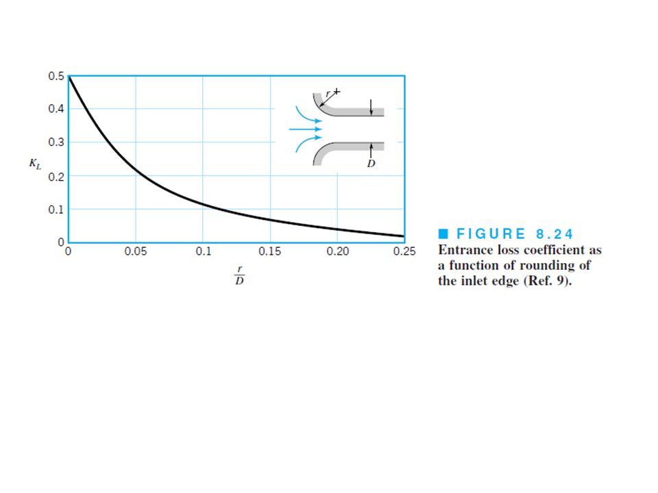
Minor losses in pipe system
Head loss in the pipe system components like valves, bends, tees, elbow sudden change in pipe cross section are considered as minor losses in pipes. Frictional losses in straight pipe portion is termed as major loss. Losses due to pipe system components are given in terms of loss coefficients(KL).
.")
28
As inertia forces dominates over the viscous forces in the pipe system components, effect of Re is negligible in most practical consideration A valve is a variable resistance element in a pipe circuit.

34
The loss coefficient for a sudden expansion can be theoretically calculated.

35
solution

36
Types of pipe flow system problems

37
Type I f from Moody chart directly or using Colebrook formula

38
Type II

39
Type III 1

40
Swamee and Jain proposed the following explicit relations in 1976 that are accurate to within 2 percent of the Moody chart:

41
solution

42
Multiple Pipe Systems Series 1 2

43
Parallel

44
Three reservoir pipe junction

45
Piping network solution scheme

48
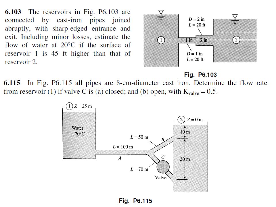
6.103

49
6.115

50
6.115

51
6.121

54
back

55
back

Similar presentations


 Chapter 9: FLOWS IN PIPE>")


