1. Summary of the Statistics used in Multiple Regression

2. The Least Squares Estimates: - The values that minimize

3. The Analysis of Variance Table Entries a) Adjusted Total Sum of Squares (SS Total ) b) Residual Sum of Squares (SS Error ) c) Regression Sum of Squares (SS Reg ) Note: i.e. SS Total = SS Reg +SS Error

4. The Analysis of Variance Table SourceSum of Squaresd.f.Mean SquareF RegressionSS Reg pSS Reg /p = MS Reg MS Reg /s 2 ErrorSS Error n-p-1SS Error /(n-p-1) =MS Error = s 2 TotalSS Total n-1

5. Uses: 1.To estimate  2 (the error variance). - Use s 2 = MSError to estimate  2. 2.To test the Hypothesis H 0 :  1 =  1 =  2 =...  =  p = 0. Use the test statistic F = MS Reg / s 2 = [(1/p)SS Reg ]/[(1/(n-p-1))SS Error ]. - Reject H 0 if F > F a (p,n-p-1).

6. 3.To compute other statistics that are useful in describing the relationship between Y (the dependent variable) and X 1, X 2,...,X p (the independent variables). a)R 2 = the coefficient of determination = SS Reg /SS Total = = the proportion of variance in Y explained by X 1, X2,...,X p 1 - R 2 = the proportion of variance in Y that is left unexplained by X 1, X2,..., X p = SSError/SSTotal.

7. b)R a 2 = "R 2 adjusted" for degrees of freedom. = 1 -[the proportion of variance in Y that is left unexplained by X 1, X 2,..., X p adjusted for d.f.] = 1 - [(1/(n-p-1))SS Error ]/[(1/(n-1))SS Total ]. = 1 - [(n-1)SS Error ]/[(n-p-1)SS Total ]. = 1 - [(n-1)/(n-p-1)] [1 - R 2 ].

8. c) R=  R 2 = the Multiple correlation coefficient of Y with X 1, X 2,...,X p = = the maximum correlation between Y and a linear combination of X 1, X 2,...,X p Comment: The statistics F, R 2, R a 2 and R are equivalent statistics.

9. Properties of the Least Squares Estimators: 1.Normally distributed ( If there error terms are Normally distributed) 2.Unbiased Estimators of the Linear Parameters  0,  1,  2,...  p. 3.Minimum Variance (Minimum Standard Error) of all Unbiased Estimators of the Linear Parameters  0,  1,  2,...  p.

10. Comments: 1.The Error Variance s 2 (and s). 2.s X i, the standard deviation of X i (the i th independent variable). 3.The sample size n. 4.The correlations between all pairs of variables.

11. decreases as s decreases. decreases as s X i increases. decreases as n increases. increases as the correlation between pairs of independent variables increases. –In fact the standard error of the least squares estimates can be extremely high if there is a high correlation between one of the independent variables and a linear combination of the remaining independent variables. (the problem of Multicollinearity). The standard error of  ˆ i, S.E.   ˆ i   s  ˆ i

12. The Covariance Matrix,Correlation and X T X inverse matrix The Covariance Matrix where and

13. The Correlation Matrix

14. The X T X inverse matrix

15. If we multiply each entry in the X T X inverse matrix by s 2 = MS Error this matrix turns into the covariance matrix for :

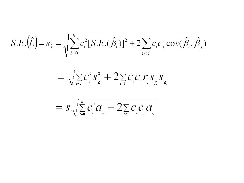
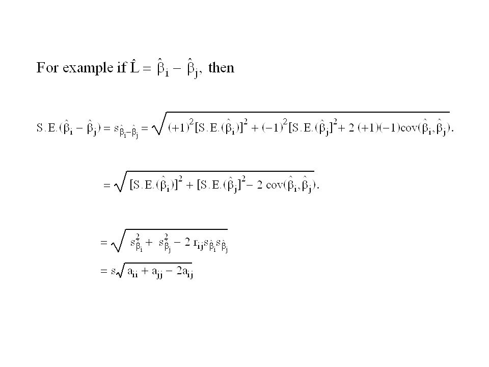
16. These matrices can be used to compute standard Errors for linear combinations of the regression coefficients Namely

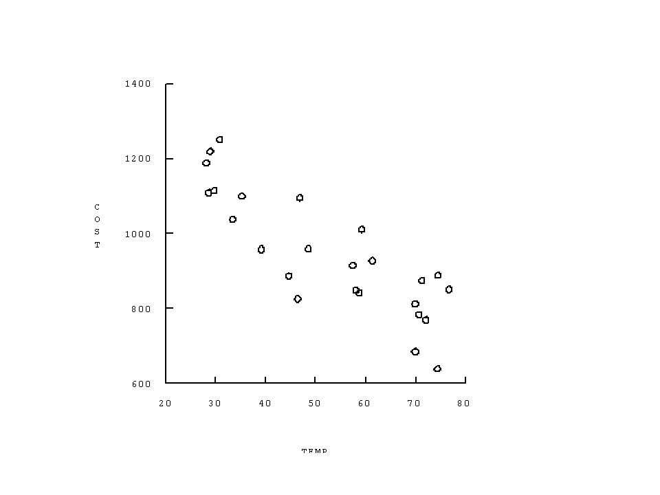
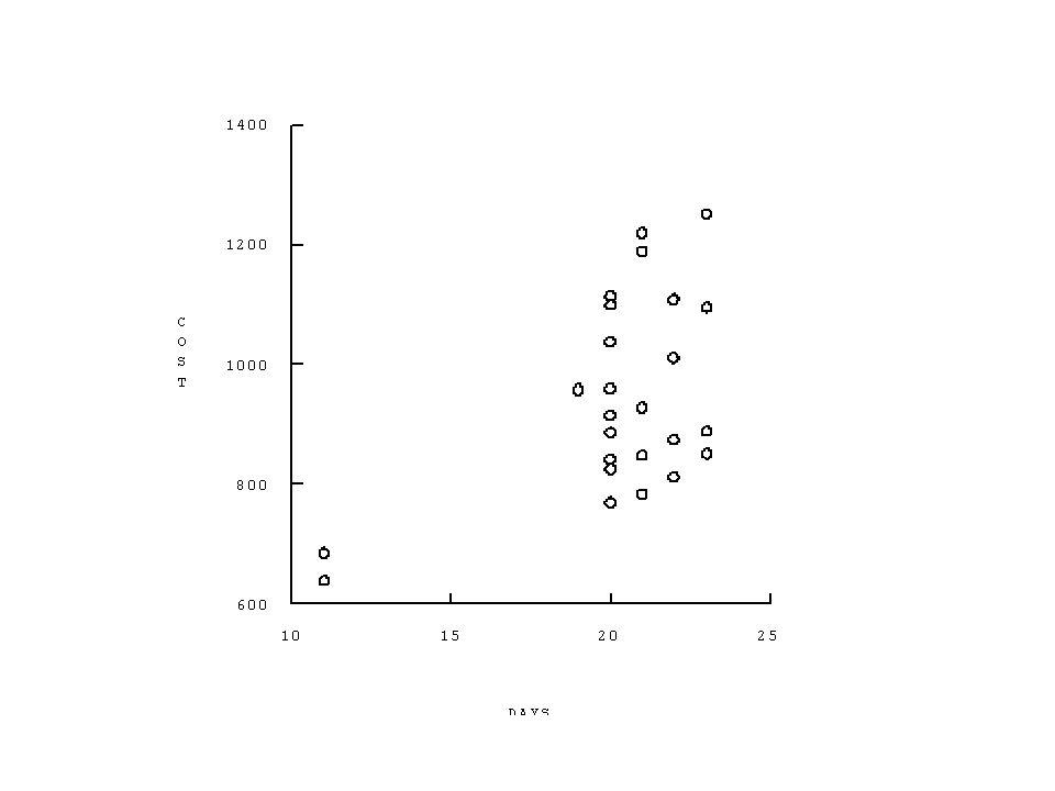
19. An Example Suppose one is interested in how the cost per month (Y) of heating a plant is determined the average atmospheric temperature in the Month (X 1 ) and the number of operating days in the month (X 2 ). The data on these variables was collected for n = 25 months selected at random and is given on the following page. Y = cost per month of heating a plant X 1 = average atmospheric temperature in the month X 2 = the number of operating days for the plant in the month.

20. The Least Squares Estimates: ConstantX1X1 X2X2 Estimate912.6-7.2420.29 Standard Error110.280.804.577 The Covariance Matrix ConstantX1X1 X2X2 12162-49.203-464.36 X1X1.63390.76796 X2X2 20.947 The Correlation Matrix ConstantX1X1 X2X2 1.000-.1764-.0920 X1X1 1.000.0210 X2X2 1.000 The X T X Inverse matrix ConstantX1X1 X2X2 2.778747-0.011242-0.106098 X1X1 0.14207x10 - 3 0.175467x10 -3 X2X2 0.478599

21. The Analysis of Variance Table SourcedfSSMSF Regression254187127093661.899 Error22962874377 Total24638158

22. Summary Statistics (R 2, R adjusted 2 = R a 2 and R) R 2 = 541871/638158 =.8491 (explained variance in Y - 84.91 %) R a 2 = 1 - [1 - R 2 ][(n-1)/(n-p-1)] = 1 - [1 -.8491][24/22] =.8354 (83.54 %) R = =.9215 = Multiple correlation coefficient

25. Three-dimensional Scatter-plot of Cost, Temp and Days.

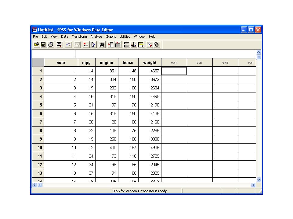
26. Example Motor Vehicle example Variables 1.(Y) mpg – Mileage 2.(X 1 ) engine – Engine size. 3.(X 2 ) horse – Horsepower. 4.(X 3 ) weight – Weight.

28. Select Analysis->Regression->Linear

29. To print the correlation matrix or the covariance matrix of the estimates select Statistics

30. Check the box for the covariance matrix of the estimates.

31. Here is the table giving the estimates and their standard errors.

32. Here is the table giving the correlation matrix and covariance matrix of the regression estimates: What is missing in SPSS is covariances and correlations with the intercept estimate (constant).

33. This can be found by using the following trick 1.Introduce a new variable (called constnt) 2.The new “variable” takes on the value 1 for all cases

34. Select Transform->Compute

35. The following dialogue box appears Type in the name of the target variable - constnt Type in ‘1’ for the Numeric Expression

36. This variable is now added to the data file

37. Add this new variable (constnt) to the list of independent variables

38. Under Options make sure the box – Include constant in equation – is unchecked The coefficient of the new variable will be the constant.

39. Here are the estimates of the parameters with their standard errors Note the agreement with parameter estimates and their standard errors as previously calculated.

40. Here is the correlation matrix and the covariance matrix of the estimates.

41. Testing for Hypotheses related to Multiple Regression. The General Linear Hypothesis H 0 :h 11  1 + h 12  2 + h 13  3 +... + h 1p  p = h 1 h 21  1 + h 22  2 + h 23  3 +... + h 2p  p = h 2... h q1  1 + h q2  2 + h q3  3 +... + h qp  p = h q where h 11  h 12, h 13,..., h qp and h 1  h 2, h 3,..., h q are known coefficients.

42. Examples 1.H 0 :  1 = 0 2.H 0 :  1 = 0,  2 = 0,  3 = 0 3.H 0 :  1 =  2 4.H 0 :  1 =  2,  3 =  4 5.H 0 :  1 = 1/2(  2 +  3 ) 6.H 0 :  1 = 1/2(  2 +  3 ),  3 = 1/3(  4 +  5 +  6 )

43. The Complete Model Y =  0 +  1 X 1 +  2 X 2 +  3 X 3 +... +  p X p +  The Reduced Model The model implied by H 0. You are interested in knowing whether the complete model can be simplified to the reduced model.

44. Testing the General Linear Hypothesis The F-test for H 0 is performed by carrying out two runs of a multiple regression package.

45. Run 1: Fit the complete model. Resulting in the following Anova Table: SourcedfSum of Squares RegressionpSS Reg Residual (Error)n-p-1SS Error Totaln-1SS Total

46. Run 2: Fit the reduced model (q parameters eliminated) Resulting in the following Anova Table: SourcedfSum of Squares Regressionp-qSS 1 Reg Residual (Error)n-p+q-1SS 1 Error Totaln-1SS Total

47. The Test: The Test is carried out using the Test Statistic where SS H 0 = SS 1 Error - SS Error = SS Reg - SS 1 Reg and s 2 = SS Error /(n-p-1). The test statistic, F, has an F-distribution with 1 = q d.f. in the numerator and 2 = n – p - 1 d.f. in the denominator if H 0 is true.

48. Distribution when H 0 is true

49. The Critical Region Reject H 0 if F > F  (q, n – p – 1) F  (q, n – p – 1)

50. The Anova Table for the Test: SourcedfSum of SquaresMean SquareF Regressionp-qSS 1 Reg [1/(p-q)]SS 1 Reg MS 1 Reg /s 2 (for the reduced model) DepartureqSS H0 (1/q)SS H0 MS H0 /s 2 from H 0 Residual n-p-1SS Error s 2 (Error) Totaln-1SS Total

51. Some Examples: Four independent Variables X 1, X 2, X 3, X 4 The Complete Model Y =  0 +  1 X 1 +  2 X 2 +  3 X 3 +  4 X 4 + 

52. 1)a)H 0 :  3 = 0,  4 = 0 (q = 2) b)The Reduced Model: Y =  0 +  1 X 1 +  2 X 2 +  Dependent Variable:Y Independent Variables: X 1, X 2

53. 2)a)H 0 :  3 = 4.5,  4 = 8.0 (q = 2) b)The Reduced Model: Y – 4.5X 3 – 8.0X 4 =  0 +  1 X 1 +  2 X 2 +  Dependent Variable:Y – 4.5X 3 – 8.0X 4 Independent Variables: X 1, X 2

54. Example Motor Vehicle example Variables 1.(Y) mpg – Mileage 2.(X 1 ) engine – Engine size. 3.(X 2 ) horse – Horsepower. 4.(X 3 ) weight – Weight.

55. Suppose we want to test: H 0 :  1 = 0 against H A :  1 ≠ 0 i.e. engine size(engine) has no effect on mileage(mpg). The Full model: Y =  0 +  1 X 1 +  2 X 2 +  1 X 3 +  (mpg) (engine)(horse) (weight) The reduced model: Y =  0 +  2 X 2 +  1 X 3 + 

56. The ANOVA Table for the Full model:

57. The reduction in the residual sum of squares = 7733.138452 - 7720.835649 = 12.30280251 The ANOVA Table for the Reduced model:

58. The ANOVA Table for testing H 0 :  1 = 0 against H A :  1 ≠ 0

59. Now suppose we want to test: H 0 :  1 = 0,  2 = 0 against H A :  1 ≠ 0 or  2 ≠ 0 i.e. engine size (engine) and horsepower (horse) have no effect on mileage (mpg). The Full model: Y =  0 +  1 X 1 +  2 X 2 +  1 X 3 +  (mpg) (engine)(horse) (weight) The reduced model: Y =  0 +  1 X 3 + 

60. The ANOVA Table for the Full model

61. The reduction in the residual sum of squares = 8299.023 - 7720.835649 = 578.1875392 The ANOVA Table for the Reduced model:

62. The ANOVA Table for testing H 0 :  1 = 0,  2 = 0 against H A :  1 ≠ 0 or  2 ≠ 0