1. More repeated measures

2. More on sphericity With our previous between groups Anova we had the assumption of homogeneity of variance With repeated measures design we still have this assumption albeit in a different form

3. More on sphericity Homogeneity of variance assumption means we want to see similar variability from group to group In other words we don’t want more or less variability in one group’s scores relative to another

4. More on sphericity We are still worried about this problem, except now it applies to difference scores between pairs of the treatment (repeated measures) under consideration In other words the variances of the differences scores created by comparing any two treatments should be roughly the same for all pairs creating difference scores

5. More on sphericity Raw data (top) Difference scores (bottom) We could then calculate variances for each of these sets of differences The sphericity assumption is that the all these variances of the differences are equal (in the population sampled). In practice, we'd expect the observed sample variances of the differences to be similar if the sphericity assumption was met. A 1 A 2 A 3 A 4 Participant 1 89124 Participant 2 611163 Participant 3 98125 etc.... A 1 -A 2 A 1 -A 3 A 1 -A 4 etc. Participant 1 -4+4 Participant 2 -5-10+3 Participant 3 +1-3+4 etc.... Var 1-2 Var 1-3 Var 1-4

6. Technical side We can check sphericity assumption using the covariance matrix – –A1-A4 equals time1- time4 or what have you Variances for individual treatments in red Samples:A 1 A 2 A 3 A 4 A1A1 105 15 A2A2 5201520 A3A3 10153025 A4A4 15202540

7. Compound symmetry is the case where all variances are equal, and all covariances are equal Not bloody likely Samples:A 1 A 2 A 3 A 4 A1A1 105 15 A2A2 5201520 A3A3 10153025 A4A4 15202540

8. Sphericity is a relaxed form of the assumption of compound symmetry It is that the sum of any two treatments’ variances minus their covariance equals a constant The constant is equal to the variance of their difference scores

9. = 10 + 20 - 2(5) = 20 = 10 + 20 - 2(5) = 20 = 10 + 30 - 2(10) = 20 = 10 + 30 - 2(10) = 20 = 10 + 40 - 2(15) = 20 = 10 + 40 - 2(15) = 20 = 20 + 30 - 2(15) = 20 = 20 + 30 - 2(15) = 20 = 20 + 40 - 2(20) = 20 = 20 + 40 - 2(20) = 20 = 30 + 40 - 2(25) = 20 = 30 + 40 - 2(25) = 20 Samples:A 1 A 2 A 3 A 4 A1A1 105 15 A2A2 5201520 A3A3 10153025 A4A4 15202540

10. SPSS You can produce the variance/ covariance matrix in SPSS repeated measures

11. Output from our previous stress data

12. More complex repeated measures As with our between groups Anova, we can also have more than one repeated measures factor 2-way repeated measures

13. Two way repeated measures Remember that a 2 factor ANOVA produces 3 elements of interest – –2 main effects and 1 interaction. If our 2 within-subject factors are A and B, the analysis will produce: – –a main effect of A (using A x Subjects as the error term) – –a main effect of B (using B x Subjects as the error term) – –a A X B interaction (using A x B x Subjects as the error term)

14. Example An experiment designed to look at the effects of therapy on self-esteem Subjects self-esteem measures 5 subjects One within-subject effect with 4 levels (weeks 1-4) Another with 2 levels (wait,therapy)

15. Data BaselineTherapy 12341234 359656117 7 121110121815 91314121015 14 4811769139 13543597

16. Data setup Now setting up this data in SPSS follows the same general system – –Each row representing a single subject The analysis itself is run in the same way as a One-Way RM design, except now we specify 2 factors. [Analyze  General Linear Model  Repeated Measures]

17. General points The interpretation follows the same logic as a One-Way RM ANOVA The error terms reflect the differences in individuals' responsiveness to the various treatments

18. Partitioning the effects Recall from the one-way RM design that our error term was a reflection of how different subjects respond differently to different treatments – –Treatment X subject interaction The variance within people was a combination of the treatment effect, the interaction w/ subjects, and random error The error term in that situation contained both the interaction effects and random error

19. Partitioning the effects In the 2-way RM we will have the same situation for main effects and the interaction Each effect will have its own error term that contains the X subject interaction + error Gist: we test the significance of any effect with an error term that involves the interaction of that effect with factor S Between subjects (S) A –Error (A x S) B –Error (B x S) A x B –Residual Error (AB x S)

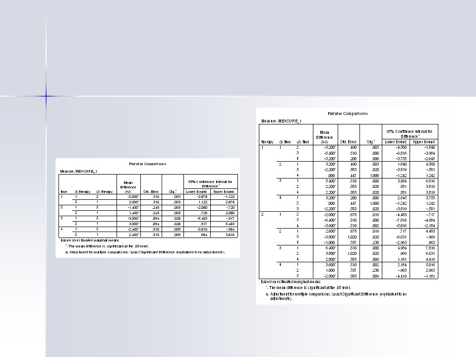
20. Results Cleaned up output from SPSS

21. Interpretation The results suggest that there is an effect of time and whether the person engages in therapy, but no statistically significant interaction We could as before perform multiple comparisons by conducting paired comparisons using an appropriate correction (e.g. B-Y) As there are only 2 levels for therapy, the main effect is the only comparison

22. Interpretation But as we noted in the factorial design, a significant interaction is not required to test for simple effects – –Plus in this case we had an interesting effect size for the interaction anyway Note that this is for demonstration only, with main effects both sig and non sig interaction you should not perform simple effects analysis. – –But even that suggestion is based on p-values so…

23. Interpretation In SPSS we can use the same emmeans function again – – /EMMEANS = TABLES(therapy*time)compare(time) – – /EMMEANS = TABLES(therapy*time)compare(therapy) The error term will be the interaction of the effect X subject at the particular level for the other within subjects factor (e.g. A x S at B 1 )

25. Another example Habituation in mice Habituation represents the simplest form of learning – –Decline in the tendency to respond to stimuli that have become familiar due to repeated exposure For example, a sudden noise may initially elicit reaction, but if we hear it repeatedly, we gradually get use to it so that we are less startled the second time we hear it and eventually just ignore it. If stimulus withheld for some period following habituation, the response will recover

26. Mice were placed in a chamber and presented with a startle tone for 50 trials, and startle response was recorded. Then they were given a 30 minute break and run again. Data broken down into 5 blocks of 10 trials each for each session, and it is the blocks that will be analyzed

27. In SPSS

28. Graphically

29. We may want to test specific pairwise comparisons Perhaps we want to know if there was a significant drop from block 1 to block 5 in session 1, which would be habituation. Then we want to look at recovery from block 5 session 1 to block 1 session 2. Then see if there is habituation in session 2. Think of it as 10 blocks of 10 trials each. – –In other words, stretch it out in a line.

30. Output

31. Contrasts Perhaps instead we wanted to test a specific type of contrast – –Recall difference, repeated, helmert etc.

32. In this example I chose a ‘simple’ contrast to test for habituation for the first session Compares each mean to some reference mean – –First block

33. More complex Your text provides an example of a 3 way repeated measures design – –Had we the trial data we could have done so for the mice example The concepts presented here extend to that without having to add any new techniques Effects: df Sn-1 Aa-1 –A x S(a-1)(n-1) Bb-1 –B x S(b-1)(n-1) Cc-1 –C x S(c-1)(n-1) A x B(a-1)(b-1) –AB x S(a-1)(b-1)(n-1) B x C(b-1)(c-1) –BC x S (b-1)(c-1)(n-1) A x C(a-1)(c-1) –A C x S (a-1)(c-1)(n-1) A x B x C(a-1)(b-1)(c-1) –ABC x S (a-1)(b-1)(c-1)(n-1)