Fourier Transform J.B. Fourier 1768-1830. Image Enhancement in the Frequency Domain 1-D Image Enhancement in the Frequency Domain 1-D.

Fourier Transform J.B. Fourier 1768-1830

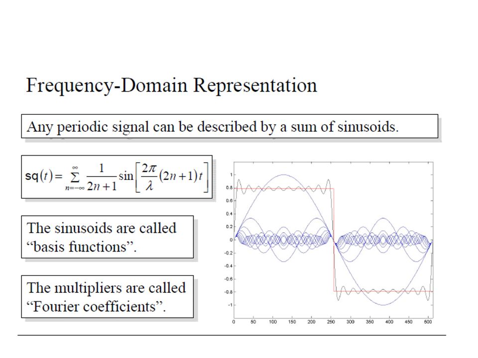
Image Enhancement in the Frequency Domain 1-D Image Enhancement in the Frequency Domain 1-D

= 3 sin(x) A + 1 sin(3x) B A+B + 0.8 sin(5x) C A+B+C + 0.4 sin(7x)D A+B+C+D A sum of sines and cosines sin(x) A

Fourier spectrum of step function

The Continuous Fourier Transform

The Fourier Transform 1D Continuous Fourier Transform: The Inverse Fourier Transform The Continuous Fourier Transform 2D Continuous Fourier Transform: The Inverse Transform The Transform

Discrete Functions 0 1 2 3... N-1 f(x) f(x 0 ) f(x 0 +  x) f(x 0 +2  x) f(x 0 +3  x) f(n) = f(x 0 + n  x) x0x0 x0+xx0+x x 0 +2  xx 0 +3  x The discrete function f: { f(0), f(1), f(2), …, f(N-1) }

(u = 0,..., N-1) (x = 0,..., N-1) 1D Discrete Fourier Transform: The Discrete Fourier Transform 2D Discrete Fourier Transform: (x = 0,..., N-1; y = 0,…,M-1) (u = 0,..., N-1; v = 0,…,M-1)

The wavelength is. The direction is u/v. The 2D Basis Functions u=0, v=0 u=1, v=0u=2, v=0 u=-2, v=0u=-1, v=0 u=0, v=1u=1, v=1u=2, v=1 u=-2, v=1u=-1, v=1 u=0, v=2u=1, v=2u=2, v=2 u=-2, v=2u=-1, v=2 u=0, v=-1u=1, v=-1u=2, v=-1 u=-2, v=-1u=-1, v=-1 u=0, v=-2u=1, v=-2u=2, v=-2 u=-2, v=-2u=-1, v=-2 U V

The Fourier Transform Jean Baptiste Joseph Fourier

1.Original: Real, imaginary, amplidute 2.F.T.; Real, imaginary, amplitude 3.Reconstructed

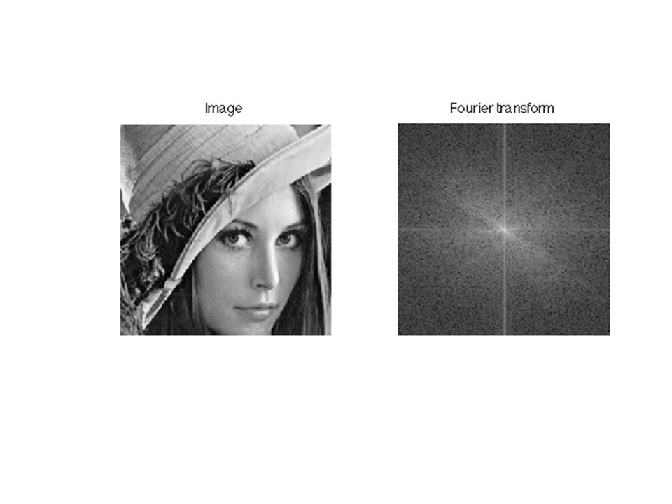
Fourier spectrum log(1 + |F(u,v)|) Image f The Fourier Image Fourier spectrum |F(u,v)|

FİLTERİNG

Frequency Bands Percentage of image power enclosed in circles (small to large) : 90%, 95%, 98%, 99%, 99.5%, 99.9% ImageFourier Spectrum

Low pass Filtering 90% 95% 98% 99% 99.5% 99.9%

Noise Removal Noisy image Fourier Spectrum Noise-cleaned image

Higher frequencies due to sharp image variations (e.g., edges, noise, etc.)

Noise Removal Noisy imageFourier SpectrumNoise-cleaned image

High Pass Filtering OriginalHigh Pass Filtered

High Frequency Emphasis + OriginalHigh Pass Filtered

High Frequency Emphasis OriginalHigh Frequency Emphasis Original High Frequency Emphasis

OriginalHigh pass Filter High Frequency Emphasis High Frequency Emphasis + Histogram Equalization High Frequency Emphasis

2D Image2D Image - Rotated Fourier Spectrum Rotation

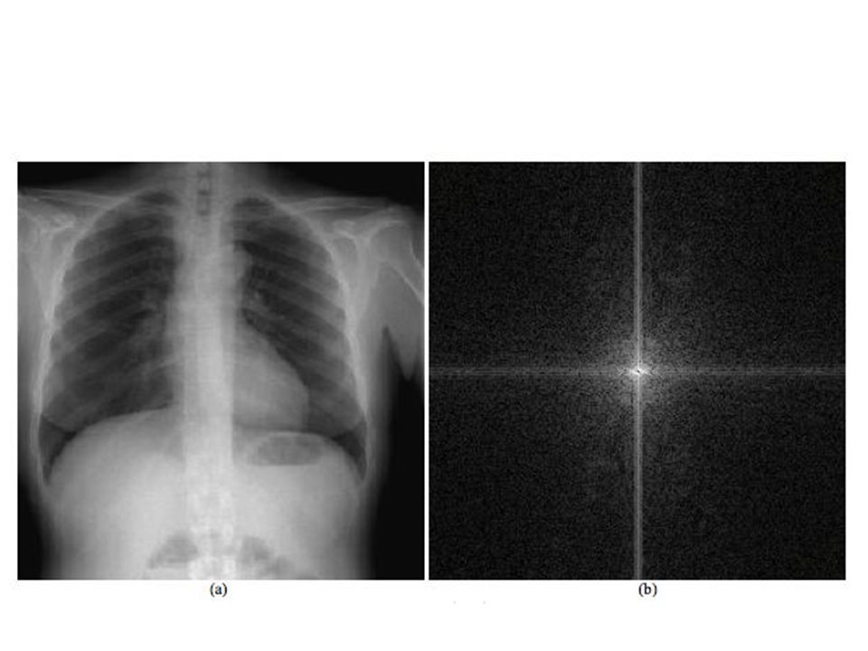
Image Domain Frequency Domain Fourier Transform -- Examples

Image Fourier spectrum Fourier Transform -- Examples

Centered Fourier Spectum

Fourier Transform of a damaged board

Low Pass and High Pass Filtering

Hihg Pass Filtering

Gaussian Filters in Frequency and Space Domains

İdeal Low pass filter

İdeal Low Pass Filter

Low Pass Filtering in freuencey Domain

Frequency Domain and Space Domain Filters

Butterworth Low Pass Filter

Filtering with different Cutoff Frequencies

Chapter 4 Image Enhancement in the Frequency Domain Chapter 4 Image Enhancement in the Frequency Domain

Remove the blackened areas in FS

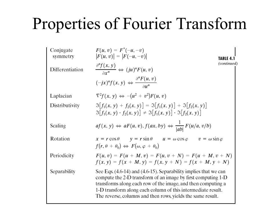
Properties of Fourier Transform

Fourier Transform Pairs

Hadamard Basis MAtrices

DCT Basis MAtrices

Wavelets

Example: 2D Haar 2D Haar scaling: 2D Haar wavelets:

Subspaces V 2 j is the two-dimensional subspace at scale j. As j increases, we get L 2 (R 2 ).

2D wavelet decomposition The approximation and detail coefficients are computed in a similar way: The reconstruction is:

Filterbank Structure: Decomposition

Filterbank Structure: Reconstruction

The Three Frequency Channels We can interpret the decomposition as a breakdown of the signal into spatially oriented frequency channels. Decomposition of frequency support Arrangement of wavelet representations

Wavelet Decomposition: Example LENA

Wavelet Example 2

Applications: Edge Detection in Images

Application: Image Denoising Using Wavelets Noisy Image:Denoised Image:

Denoising Images Denoising Daubechies’ face: –Transform the image to the wavelet domain –Apply a threshold at two standard deviations –Inverse-transform the image.

Image Denoising Using Wavelets Calculate the DWT of the image. Threshold the wavelet coefficients. The threshold may be universal or subband adaptive. Compute the IDWT to get the denoised estimate. Soft thresholding is used in the different thresholding methods. Visually more pleasing images.

Image Enhancement Image contrast enhancement with wavelets, especially important in medical imaging Make the small coefficients very small and the large coefficients very large. Apply a nonlinear mapping function to the coefficients.

Experiments

Denoising and Enhancement Apply DWT Shrink transform coefficients in finer scales to reduce the effect of noise Emphasize features within a certain range using a nonlinear mapping function Perform IDWT to reconstruct the image.

Examples Original Denoised Denoising with Enhancement

Edge Detection Edges correspond to the singularities in the image and are related to the local maxima of wavelet coefficients. For edge detection, a smoothing function (such as a spline) and two wavelet functions are defined. Wavelet functions are usually the first and second order derivatives of the smoothing function. Examples: Keep the detail coefficients and discard the approximation coefficients Edges correspond to large coefficients

Applications Computer vision Image processing in the human visual system has a complicated hierarchical structure that involves several layers of processing. At each processing level, the retinal system provides a visual representation that scales progressively in a geometrical manner. Intensity changes occur at different scales in an image, so that their optimal detection requires the use of operators of different sizes. Therefore, a vision filter have two characteristics: it should be a differential operator, and it should be capable of being tuned to act at any desired scale. Wavelets are ideal for this

FBI Fingerprint Compression A single fingerprint is about 700,000 pixels, and requires about 0.6MBytes.

Image Compression and Wavelets

Why Compression? Uncompressed images take too much space, require larger bandwidth for transmission and longer time to transmit Examples: –512x512 grayscale image: 262KB –512x512 color image: 786KB The common principle beyond compression is to reduce redundancy: spatial and spectral redundancy

Types of Compression Lossy vs. Lossless: Lossy compression discards redundant information, achieves higher compression ratios. Lossless compression can reconstruct the original image. Predictive vs. Transform Coding

Components of a Coder Source Encoder: Transform the image –DFT,DCT,DWT (linear transforms) Quantizer: Scalar vs. Vector (lossy coding) Entropy Encoder: Compresses the quantized values (lossless)

Original JPEG Use DCT to transform the image (real part of DFT)

Original JPEG Transform each 8x8 block using DCT Since adjacent pixels are highly correlated, most of the coefficients are concentrated at lower frequencies. Quantize the DCT coefficients (uniform quantization) and then entropy encode for further compression

Disadvantages of DCT: Why wavelets? DCT based JPEG uses blocks of image, there is still correlation across blocks. Block boundaries are noticeable in some cases Blocking artifacts at low bit rates Can overlap the blocks  Computationally expensive

Digital Image Processing, 2nd ed. www.imageprocessingbook.com © 2002 R. C. Gonzalez & R. E. Woods Was JPEG not good enough? JPEG is based on DCT. Equal subbands. At low bit rates, there is a sharp degradation with image quality. 43:1 compression ratio

Why Wavelets? No need to block the image More robust under transmission errors Facilitates progressive transmission of the image (Scalability)

Features of JPEG2000 Multiple Resolution: Decomposes the image into a multiple resolution representation. Progressive transmission: By pixel and resolution accuracy, referred to as progressive decoding and signal-to-noise ratio (SNR) scalability: This way, after a smaller part of the whole file has been received, the viewer can see a lower quality version of the final picture. Lossless and lossy compression Random code-stream access and processing: JPEG 2000 supports spatial random access or region of interest access at varying degrees of granularity. This way it is possible to store different parts of the same picture using different quality. Error resilience: JPEG 2000 is robust to bit errors introduced by noisy communication channels, due to the coding of data in relatively small independent blocks.

JPEG2000 Basics General block diagram of the JPEG 2000 (a) encoder and (b) decoder

Wavelets in Image Coding Orthogonal vs. Biorthogonal: –JPEG 2000 uses biorthogonal filters –Lossless and lossy compression –Cohen-Daubechies-Feavau filters 9/7 –CDF 5/3 for lossless compression (integer) –Filters are symmetric/anti-symmetric –Nearly orthogonal –Symmetric extensions of the input data

Steps in JPEG2000 Tiling: The image is split into tiles, rectangular regions of the image that are transformed and encoded separately. Tiles can be any size. Dividing the image into tiles is advantageous in that the decoder will need less memory to decode the image and it can opt to decode only selected tiles to achieve a partial decoding of the image. Using many tiles can create a blocking effect. Wavelet Transform: Either CDF 9/7 or CDF 5/3 biorthogonal wavelet transform. Quantization: Scalar quantization Coding: The quantized subbands are split into precincts, rectangular regions in the wavelet domain. They are selected in a way that the coefficients within them across the sub-bands form approximately spatial blocks in the image domain. Precincts are split further into code blocks. Code blocks are located in a single sub-band and have equal sizes. The encoder has to encode the bits of all quantized coefficients of a code block, starting with the most significant bits and progressing to less significant bits by EBCOT scheme.

DWT for Image Compression Image Decomposition –Parent –Children –Descendants: corresponding coeff. at finer scales –Ancestors: corresponding coeff. at coarser scales HL 1 LH 1 HH 1 HH 2 LH 2 HL 2 HL 3 LL 3 LH 3 HH 3 –Parent-children dependencies of subbands: arrow points from the subband of parents to the subband of children.

DWT for Image Compression Image Decomposition –Feature 1: Energy distribution concentrated in low frequencies –Feature 2: Spatial self-similarity across subbands HL 1 LH 1 HH 1 HH 2 LH 2 HL 2 HL 3 LL 3 LH 3 HH 3 The scanning order of the subbands for encoding the significance map.

DWT for Image Compression Differences from DCT Technique – In conventional transform coding: Anomaly (edge) produces many nonzero coeff. insignificant energy TC allocates too many bits to “trend”, few bits left to “anomalies” Problem at Very Low Bit-rate Coding : block artifacts –DWT Trends & anomalies information available Major difficulty: fine detail coefficients associated with anomalies  the largest no. of coeff. Problem: how to efficiently represent position information?

112 2-D WT Example Boats image WT in 3 levels

113 WT-Application in Denoising Boats image Noisy image (additive Gaussian noise)

114 WT-Application in Denoising Boats image Denoised image using hard thresholding

DWT for Image Compression Differences from DCT Technique – In conventional transform coding: Anomaly (edge) produces many nonzero coeff. insignificant energy TC allocates too many bits to “trend”, few bits left to “anomalies” Problem at Very Low Bit-rate Coding : block artifacts –DWT Trends & anomalies information available Major difficulty: fine detail coefficients associated with anomalies  the largest no. of coeff. Problem: how to efficiently represent position information?

Fourier Transform J.B. Fourier 1768-1830. Image Enhancement in the Frequency Domain 1-D Image Enhancement in the Frequency Domain 1-D.

Similar presentations

Presentation on theme: "Fourier Transform J.B. Fourier 1768-1830. Image Enhancement in the Frequency Domain 1-D Image Enhancement in the Frequency Domain 1-D."— Presentation transcript:

Similar presentations

About project

Feedback

Log in

Auth with social network:

Fourier Transform J.B. Fourier 1768-1830. Image Enhancement in the Frequency Domain 1-D Image Enhancement in the Frequency Domain 1-D.

Similar presentations

Presentation on theme: "Fourier Transform J.B. Fourier 1768-1830. Image Enhancement in the Frequency Domain 1-D Image Enhancement in the Frequency Domain 1-D."— Presentation transcript:

Similar presentations

About project

Feedback