1. 1 Results for OMPS NP OMPS NPP ST Meeting 8/15/2013 L. Flynn (STAR) with contributions from Wei Yu, Jiangou Niu, Zhihua Zhang, Eric Beach, Trevor Beck and Chunhui Pan

2. Outline  Solar Measurements (In separate PDF NP_SOL_fit.pdf)  Stray Light Effects on Layer Ozone  Initial Measurement Residual Time Series  Chasing Orbit comparisons between OMPS and NOAA-19  Monthly Average Retrieved minus A Priori for NOAA-16 and NOAA-19 SBUV/2 and OMPS NP V8  Monitoring figures are available at http://www.star.nesdis.noaa.gov/icvs/PROD/proOMPSbeta.O 3PRO_V8.php 2

3. Description of results in NP_SOL_fit.pdf The first analysis was designed to find the scale factors, the wavelength shifts, and the trends in the Working Diffuser Solar measurements. We can now use the scale factors and the wavelength shift pattern to see how the reference diffuser measurements compare. (We can also check to see if the wavelength shifts are in common between the working and reference.) I agree that even without this analysis the reference spectra evolution looks fairly flat which implies that the trend is mainly from changes in the Working Diffuser, not the instrument throughput. That may not be the entire case. Since the reference measurements are paired with working measurements close in time, we can also compute the relative trends with just two pairs as is done in the second set of results in the figure on bottom of Page 3. We've continued the analysis with both working and reference. We first normalize the spectra by using the average of the working measurements Nsolar(w,t) = Solar(w,t)/AWSolar(w) - 1. We then compute an estimate of the wavelength shift pattern by using quadratic fits of three consecutive AWSolar(w) values and taking the slope at the midpoint as an estimate of the change in radiance per pixel shift. We then normalize these value to make them relative shifts. This gives us a shift(w) pattern. We then fit each Nsolar(w) with shift(w) to get a single shift estimate for each full spectrum relative to the average one. The first page of the attached files shows the relative shift pattern as %/one-pixel-shift on the top plot, and the shifts for each spectrum on the bottom plot. The three *'s are for the Reference Diffuser. There is good agreement in the timing of the shifts between the Working, +'s, and Reference even though the Working spectra are used to find the normalizing spectrum and shift pattern. Notice the suggestion of an annual cycle in the wavelength shifts. Multiple regression is now used for the normalized, shift-removed spectra including both Working and Reference. The model is NSRSolar(w,t) = HW*c1(w)*t + c2(w)*mg2(t) + HW*c3(w) + HR*c4(w)*t + HR*c5(w) where HW is 1 for working diffuse measurements and 0 for reference and HR is the opposite, and the Mg2 Indices are proportional changes relative to the average (the Mg II indices for the Reference were adjusted to remove a bias with the working index computations.) The Mg II scale factors, c2(w) term from the regression model, are in the top plot on Page 2. The Mg II indices, mg2(t) term from the model, are in the bottom plot. Notice that the Reference Diffuser measurements are taken at times with very different solar activity. The third page shows the trend terms from the model on the top figure. The upper line is the Reference Diffuser trend term, c4(w), and the lower line is the Working Diffuser trend term, c1(w). If we assume that the reference diffuser is stable, then the c4(w) pattern represents instrument throughput changes. The lower plot shows the difference in the Working and Reference trends, c1(w)-c4(w). The dotted line is the simple direct calculation one can do with double difference of the Day 81 paired diffuser measurements versus the Day 450 pair, namely, Work(w,450)/Work(w,81) - Ref(w,450)/Ref(w,81). The fourth page just shows the two constant terms from the multiple regression; working, c3(w), on the top and reference, c5(w), on the bottom. These are related to the choice of a Day 0, the use of the Mg II Index average to get deviations, and the use of the Working diffuser average for the normalization. The plot on the top of the fifth page shows the measurements and model results for the 11th wavelength. All the spectra were normalized by the average for the 29 working measurements. The data values in this figure are also after the wavelength shift adjustments have been applied. While one would expect that the three reference measurements (+ measured; * modeled) shown here would give a slightly positive trend, the two later measurements occur at peaks in the solar activity. The dashed lines show the measured data if we adjust for solar activity, that is, subtract the c2(w)*mg2(t) term. The change for the three reference data points is dramatic. The bottom figure on the fifth page shows sample spectra and models for the working diffuser. The spectra have been normalized relative to the working average and the wavelength shift adjustment has been applied. The sixth page shows sample spectra and models for the working diffuser (top figure) and reference diffuser (bottom figure). Both spectra are normalized but without the wavelength shift applied. They are compared to the model plus the fit wavelength shift. The model in the lower figures includes the separate offset (to account for the use of the working average as normalization) and trend calculations for the reference spectra. 3

4. Description of analysis and results for NP Solar Measurements The OMPS Nadir Profiler Solar measurements were analyzed to investigate changes over the first year of measurements. A total of thirty-two spectra with three from the reference diffuser (on March 21, 2012, August 31, 2012 and April 1, 2013) and 29 from the working diffuser (taken approximately every two weeks from March 7, 2012 to April 1, 2013) were used in the study. The spectra are taken at 147 wavelengths from 250 to 310 nm. For each measurement for each wavelength, the values are averaged over the spatial dimension of the CCD array (100 pixels). The initial analysis found three types of changes in the spectra as follows: those related to solar activity as we pass through the peak of Solar Cycle 24; those related to wavelength scale shifts most likely produced by annual variations in the instrument optical bench or aperture temperatures at the orbital locations of the measurements; and decreases in the measured irradiance values probably produced by uncorrected changes in the instrument throughput or diffuser properties over time. A model of the measurements was devised using three assumptions corresponding to the observed variations. For the first component, it was assume that the solar irradiance variations could be modeled by using a Mg II core-to-wing ratio and scale factors as described in Deland and Cebula (1993). That is, that a ratio of the measurements at the center of the Mg II feature at 280 nm to the measurements at the wings on either side would be a good proxy for solar activity and that a single wavelength pattern of scale factors could accurately predict the variations of a full spectrum from a variation in the Mg II Index. For the second component, it was assumed that relative shape of the variations produced by a spectral scale shift could be found by examining the average solar spectrum variations. Specifically, three consecutive measurements of the average spectrum were fit with a quadratic and the slope of the quadratic at the central point was used as an estimate of the effects of shift at that wavelength. These were normalized by the average spectrum values and the wavelength spacing to produce a relative change pattern with units of 0.4 nm^-1 (1/pixel spectral spacing). For the trend components simple linear trends in time were used with separate terms for the working and reference measurements. (Exponential models are often used to represent degradation but for small changes these are well approximated by linear terms.) The working diffuser exposure time grew at fairly consistent rate over this time period as there was a regular schedule of measurements. This means that calendar time is a good proxy for exposure time. Two sets of constants terms were also included as the working and reference spectra show a small, wavelength-dependent pattern of offsets. The model components are estimate in three steps. First a set of Mg II Index values are computed by fitting quadratics to three subsets of five irradiance values each centered at 277, 280 and 283 nm. The irradiance values at the vertices of these are used as the lower wing, core and upper wing values in the index. This gives two sets of indices. Mg2W(t) and Mg2R(t) for the working and reference diffusers on day t. (The wavelength coordinate of the vertices for the central fit tracks well with the wavelength scale shift values as found with the approach in the next paragraph. There are some small differences in the results depending on whether one removes the wavelength scale shifts before finding the Mg II Index values or removes the solar activity before finding the wavelength shifts.) The Mg II Index variations from OMPS also track well with variations of Mg II Indices from other satellite sources, e.g., MetOp-A GOME-2, over this period. Next a wavelength scale shift relative to the average spectrum is found by taking the relative differences of each spectrum with the average and finding the least squares fit of those differences with the spectral shift pattern described above. The fit is then removed to create a set of spectra with consistent wavelength scales. (You could include figure showing annual cycle in shift quantities in units of 1/pixel separation) SolarWS(w,t) = SolarW(w,t) – Shift(t)*Shift(w) SolarRS(w,t) = SolarR(w,t) – Shift(t)*Shift(w) Where SolarW(w,t) is the normalized irradiance spectrum for the working diffuser on day t (measured since January 1, 2012) and SolarR(w,t) is the same for the reference diffuser. These adjusted relative spectra were now used in multiple linear regression models of the form SolarWS(w,t) = c1(w)*t + c2(w)*Mg2W(t) + c3(w) SolarRS(w,t) = c4(w)*t + c2(w)*Mg2W(t) + c5(w) to obtain estimates of the trends and scale factors. This model is applied for each wavelength, w, individually. Note that the solar activity terms are shared but the trends and offsets are found independently for each diffuser. Ref: Matthew T. DeLand, Richard P. Cebula, “Composite Mg II solar activity index for solar cycles 21 and 22,” Journal of Geophysical Research: Atmospheres (1984–2012), Volume 98, Issue D7, pages 12809–12823, 20 July 1993, DOI: 10.1029/93JD00421 4

5. Scatter Plots of Ozone Layer Variations versus Reflectivity Variations for the first five orbits of May 15, 2013 5

6. V8 Equatorial Zonal Mean Initial Residual Time Series 6 IDPS SDR does not have dark current correction until 2/2013 Weekly Dark Updates Began Soft Calibration Adjustment

7. 7 V6 Equatorial Zonal Mean Initial Residual Time Series IDPS SDR does not have dark current correction until 2/2013 252 nm Channel not turned on for OMPS NP

8. 8 Weekly Dark Updates Began Soft Calibration Adjustment

9. Well-matched Orbits for November 29

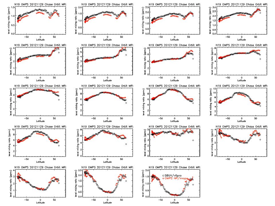
10. Profile Comparisons between OMPS & SBUV/2 V6Pro The figures on the next slides show comparisons of the ozone profile retrievals estimates between IMOPO and the NOAA-19 SBUV/2 processed with the Version 6 ozone profile retrieval algorithm. The data are from another single pair of orbits on March 6, 2013 where the two satellites are flying in formation (orbital tracks within 50 KM and sensing times with 10 minutes). The next slide compares the ozone profile retrievals in 12 pressure layers in Dobson Units versus Latitude. The 12 layers are defined by the following 13 layer boundaries: [0.0,0.247,0.495,0.99,1.98,3.96,7.92,15.8,31.7,63.3,127.0,253.0,1013] hPa. The top three layers’ results are in the top row with the topmost layer on the upper left. The lowest layer’s results are in the figure on the bottom right. The OMPS Nadir Profiler values are in Red and the SBUV/2 are shown in Black. A significant number of the OMPS Nadir Profilers contain fill values because of Error Codes incorrectly set to 20. The second slide shows the results of comparison for the ozone mixing ratios at 19 pressure levels: [0.3,0.4,0.5,0.7,1.0,1.5,2.0,3.0,4.0,5.0,7.0,10.,15.,20.,30.,40.,50.,70.,100.] hPa. The arrangement from top to bottom follows the same convention as for the layers. The two sets of figures show similar results with general agreement between the retrievals for the two instruments but with the OMPS NP retrieving much smaller values at the top of the profiles. This is probably due to the inaccuracies in the initial calibration of the shorter wavelength channels but could also be symptomatic of stray light in the shorter wavelength channels providing information at those levels.

11. Chasing orbit comparisons of SBUV/2 and OMPS-NP Version 6 Ozone Profiles 11

12. Chasing orbit comparisons of SBUV/2 and OMPS-NP Version 6 Initial Measurement Residuals 12

13. The OMPS Nadir Profiler values are in Red and the SBUV/2 are shown in Black.

15. V8 Retrieved minus A Priori for July 2013 15