1. Chapter 6 Discrete-Time System

2. 2/90  Operation of discrete time system 1. Discrete time system where and are multiplier D is delay element Fig. 6-1.

3. 3/90 2. Difference equation  Difference equation where and is constant or function of n

4. 4/90  Example 6-1 –Moving average  Example 6-2 –Integration If

5. 5/90  Functional relationship of discrete time system 3. Linear time-invariant system where is impulse response of system Fig. 6-2.

6. 6/90 –The system is said to be linear if –The system is said to be time-invariant if

7. 7/90  Form and transfer function –Difference equation of discrete time system After z-transform

8. 8/90 –Transfer function If where is impulse response of system

9. 9/90 –Impulse response of discrete time system If is power series In this case,

10. 10/90  Example 6-3 Using power series

11. 11/90 Using other method Substitute, and initial value

12. 12/90  Example 6-4 Using z-transfrom Using inverse z-transfrom

13. 13/90 If initial value Using inverse z-transfrom

14. 14/90  System stability –BIBO(bounded input, bounded output)

15. 15/90  Raible tabulation Table 6-1. Raible’s tabulation

16. 16/90 –If part or all factor is 0 in the first row, then this table is ended Singular case –Using substitution » n th order case

17. 17/90  Example 6-5

18. 18/90  Example 6-6

19. 19/90 –Singular case

20. 20/90  Example 6-7

21. 21/90  Discrete time system transfer function H(z) 4. Description of Pole-Zero where K is gain Zeros of at : Poles of at :

22. 22/90 –Description of pole and zero in z-plane Fig. 6-3.

23. 23/90  Example 6-8 Fig. 6-4.

24. 24/90  Example 6-9 K=0.2236 Fig. 6-5.

25. 25/90  Frequency response of system –Method for calculation –Method for geometric calculation 5. Frequency response

26. 26/90  Example 6-10 Method for calculation –Substitution of and using Euler’s formular

27. 27/90 –Substitution of –

28. 28/90 Fig. 6-6.

29. 29/90 Method for geometric calculation Magnitude response Phase response Fig. 6-7.

30. 30/90 6. Realization of system Unit delay Adder/subtractor Constant multiplier Branching Signal multiplier Fig. 6-8.

31. 31/90  Direct form –Direct form 1

32. 32/90 Fig. 6-9. (a) (b)

33. 33/90 –Direct form 2 Inverse transform poles zeros

34. 34/90 Fig. 6-10. (a) (b)

35. 35/90  Example 6-11 –Direct form 1 –Direct form 2

36. 36/90 Fig. 6-11. (a) (b)

37. 37/90  Quantization effect of parameters –Quantization error of parameters Input signal quantization Accumulation of arithmetic roundoff errors Coefficient of transfer function quantization

38. 38/90  Cascade and parallel canonic form –Cascade canonic form or series form first order second order

39. 39/90 Fig. 6-12. Fig. 6-13. (a) (b)

40. 40/90 –Parallel canonic form first order second order

41. 41/90 Fig. 6-14.

42. 42/90 Fig. 6-15. (a) (b)

43. 43/90  Example 6-12 –Cascade canonic form Quantization error of parameter is decreased

44. 44/90 –Parallel canonic form

45. 45/90 Fig. 6-16. (a) (b)

46. 46/90  Example 6-13 Fig. 6-17.

47. 47/90  Example 6-14 Substitute

48. 48/90 Fig. 6-18.

49. 49/90  FIR system –Direct form Tapped delay line structure or transversal filter Fig. 6-19.

50. 50/90 –Cascade canonic form where Fig. 6-20.

51. 51/90 –Linear phase FIR system structure N is even : type 1 and type 3 or

52. 52/90 –Type 1 –Type 3 N is odd : type 2 and type 4 –Type 2 –Type 4

53. 53/90 Fig. 6-21. (a) (b)

54. 54/90  Lattice structure –Lattice structure of FIR filter Difference equation Error between and FIR filter use linear predictor where is prediction coefficient

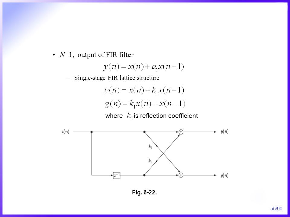
55. 55/90 N=1, output of FIR filter –Single-stage FIR lattice structure where is reflection coefficient Fig. 6-22.

56. 56/90 N=2 Fig. 6-23.

57. 57/90 N=3 Substitution Fig. 6-24.

58. 58/90 M-stage lattice structure If

59. 59/90 –Calculating filter coefficient »m-stage

60. 60/90 Fig. 6-25.

61. 61/90  Example 6-15 (1)

62. 62/90 (2) Fig. 6-26.

63. 63/90  Example 6-16 – in example 6-15

64. 64/90 –Generalization of calculating filter coefficient »Substitute for

65. 65/90 »At

66. 66/90 Divided by

67. 67/90  Example 6-17 –

68. 68/90 –Calculating of coefficient At

69. 69/90 At

70. 70/90 –Calculation of Go first stage

71. 71/90 Fig. 6-27.

72. 72/90 –Lattice structure of IIR filter All-pole system Difference equation

73. 73/90 –N=1 Fig. 6-28.

74. 74/90 –N=2 Fig. 6-29.

75. 75/90 –N th order Fig. 6-30.

76. 76/90 General IIR system function All-pole lattice structure Ladder structure

77. 77/90 –Lattice-ladder structure »System output »System transfer function

78. 78/90 where

79. 79/90 Fig. 6-31.

80. 80/90  Example 6-18 Fig. 6-32.

81. 81/90  Example 6-19 –Equation for each node

82. 82/90 Comparison of coefficients

83. 83/90 Fig. 6-33.

84. 84/90 –Advantage of digital filter compare with analog filters Digital filter can have a truly linear phase response The performance of digital filters does not vary with environmental change The frequency response of a digital filter can be automatically adjusted if it is implemented using a programmable processor Several input signals or channels can be filtered by one digital filter without the need to replicate the hardware Both filtered and unfiltered data can be saved for further use 7. Introduction to digital filter

85. 85/90 Advantage can be readily taken of the tremendous advancement in VLSI technology to fabricate digital filters and to make them small in size, to consume low power, and to keep the cost down In practice, the precision achievable with analog filters is restricted The performance f digital filters is repeatable from unit to unit Digital filters can be used at very low frequencies

86. 86/90 –Disadvantage of digital filters compare with analog filters Speed limitation Finite wordlength effect Long design and development times –Block diagram of digital filter with analog input and output Fig. 6-34.

87. 87/90  Types of digital filters : FIR and IIR filters –IIR filter –FIR filter

88. 88/90 –IIR filtering equation is expressed in recursive form –Alternative representations for FIR and IIR filters where and are coefficient of filters IIR is feedback system of some sort These transfer functions are very useful in evaluating their frequency responses

89. 89/90  Choosing between FIR and IIR filters –Relative advantages of the two filter type FIR filters can have an exactly linear phase response FIR filters are always stable. The stability of IIR filters cannot always be guaranteed The effect of using a limited number of bits to implement filters such as roundoff noise and coefficient quantization errors are much less severe in FIR than in IIR FIR requires more coefficients for sharp cutoff filters than IIR Analog filters can be readily transformed into equivalent IIR digital filters meeting similar specifications In general, FIR is algebraically more difficult to synthesize

90. 90/90 –Guideline on when to use FIR or IIR Use IIR when the only important requirements are sharp cutoff filters and high throughput Use FIR if the number of filter coefficients is not too large and, in particular, if little or no phase distortion is desired