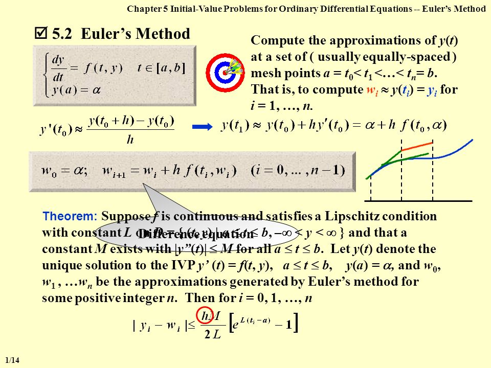
2. 1/14  5.2 Euler’s Method Compute the approximations of y(t) at a set of ( usually equally-spaced ) mesh points a = t 0 < t 1 <…< t n = b. That is, to compute w i  y(t i ) = y i for i = 1, …, n. Chapter 5 Initial-Value Problems for Ordinary Differential Equations -- Euler’s Method Difference equation Theorem: Suppose f is continuous and satisfies a Lipschitz condition with constant L on D = { (t, y) | a  t  b, –  < y <  } and that a constant M exists with |y”(t)|  M for all a  t  b. Let y(t) denote the unique solution to the IVP y’ (t) = f(t, y), a  t  b, y(a) = , and w 0, w 1, …w n be the approximations generated by Euler’s method for some positive integer n. Then for i = 0, 1, …, n

3. Chapter 5 Initial-Value Problems for Ordinary Differential Equations -- Euler’s Method Note: y”(t) can be computed without explicitly knowing y(t).  The roundoff error +  0 +  i+1 Theorem: Let y(t) denote the unique solution to the IVP y’ (t) = f(t, y), a  t  b, y(a) = , and w 0, w 1, …w n be the approximations obtained using the above difference equations. If |  i | <  for i = 0, 1, …, n, then for each i 2/14

4. Chapter 5 Initial-Value Problems for Ordinary Differential Equations -- Higher Order Taylor Methods  5.3 Higher Order Taylor Methods Definition: The difference method w 0 =  ; w i+1 = w i + h  ( t i, w i ), for each i = 0, 1, …, n – 1 has local truncation error for each i = 0, 1, …, n – 1. Note: The local truncation error is just (y i+1  w i+1 )/h with the assumption that w i = y i Note: The local truncation error is just (y i+1  w i+1 )/h with the assumption that w i = y i.  The local truncation error of Euler’s method Method of order 1 3/14

5. Chapter 5 Initial-Value Problems for Ordinary Differential Equations -- Higher Order Taylor Methods Note: Euler’s method can be derived by using Taylor’s expansion with n = 1 to approximate y(t).  Higher Order Taylor Methods Taylor method of order n: where The local truncation error is O(h n ) if y  C n+1 [a, b]. 4/14

6. Chapter 5 Initial-Value Problems for Ordinary Differential Equations -- Higher Order Taylor Methods Example: Apply Taylor’s method of order 2 and 4 to the IVP y’ = y – t 2 + 1, 0  t  2, y(0) = 0.5 Solution: Find the first 3 derivatives of f f(t, y(t)) = y(t) – t 2 + 1 f ’(t, y(t)) = y’(t) – 2t = y(t) – t 2 + 1 – 2t f ”(t, y(t)) = y’(t) – 2t – 2 = y(t) – t 2 – 2t – 1 f (3) (t, y(t)) = y’(t) – 2t – 2 = y(t) – t 2 – 2t – 1 T (2) (t i, w i ) = Taylor’s method of order 2: Given n = 10, thenh = 0.2 and t i = 0.2i w i+1 = 1.22w i – 0.0088i 2 – 0.008i + 0.22 Table 5.3 on p.269 HW: p.271 #5 (a)(b) 5/14

7.  Other Euler’s Methods  Implicit Euler’s method )(,()()()( 11101 tytfhty’htyty    )1,...,0(),(; 1110   niwtfhwww iiii  Chapter 5 Initial-Value Problems for Ordinary Differential Equations -- Higher Order Taylor Methods Usually w i+1 has to be solved iteratively, with an initial value given by the explicit method.  The local truncation error of the implicit Euler’s method Hey! Isn’t the local truncation error of Euler’s method ? Seems that we can make a good use of it … 6/14

8. Chapter 5 Initial-Value Problems for Ordinary Differential Equations -- Higher Order Taylor Methods  Trapezoidal Method Note: The local truncation error is indeed O(h 2 ). However an implicit equation has to be solved iteratively.  Double-step Method Two initial points are required to start moving forward. Such a method is called double-step method. All the previously discussed methods are single-step methods. Note: If we assume that w i – 1 = y i– 1 w i = y i he local truncation error is O(h 2 ). Note: If we assume that w i – 1 = y i – 1 and w i = y i, the local truncation error is O(h 2 ). 7/14

9. Chapter 5 Initial-Value Problems for Ordinary Differential Equations -- Higher Order Taylor Methods Method  Euler’s explicit Euler’s implicit Trapezoidal Double-step SimpleLow order accuracy stable Low order accuracy and time consuming More accurateTime consuming More accurate, and explicit Requires one extra initial point Can’t you give me a method with all the advantages yet without any of the disadvantages? Do you think it possible? Well, call me greedy… OK, let’s make it possible. 8/14

10. Chapter 5 Initial-Value Problems for Ordinary Differential Equations -- Higher Order Taylor Methods  Modified Euler’s Method Step 1: Predict a solution by the explicit Euler’s method ),( 1 iiii wtfhww   Step 2: Correct w i+1 by Plugging it into the right hand side of the trapezoidal formula )],(),([ 2 111   iiiiii wtfwtf h ww Note: This kind of method is called the predictor-corrector method. This modified Euler’ method is a single-step method of order 2. It is simpler than the implicit methods and is more stable that the explicit Euler’s method. 9/14

11. Chapter 5 Initial-Value Problems for Ordinary Differential Equations -- Runge-Kutta Methods  5.4 Runge-Kutta Methods A single-step method with high-order local truncation error without evaluating the derivatives of f. In a single-step method, a line segment is extended from (t i, w i ) to reach the next point (t i+1, w i +1 ) according to some slope. We can improve the result by finding a better slope. Idea  Check the modified Euler’s method: Must the slope be the average of K 1 and K 2 ? Must the step size be h? 10/14

12. Chapter 5 Initial-Value Problems for Ordinary Differential Equations -- Runge-Kutta Methods Generalize it to be: ),( ),( ][ 12 1 22111 phKwphphtfK wtfK KKhww ii ii ii     Determine 1, 2, and p such that the method has local truncation error of order 2. Step 1: Write the Taylor expansion of K 2 at ( t i, y i ) : Step 2: Plug K 2 into the first equation Step 3: Find 1, 2, and p such that  i+1 = ( y i+1 – w i+1 )/h = O(h 2 ). 11/14

13. Chapter 5 Initial-Value Problems for Ordinary Differential Equations -- Runge-Kutta Methods Here are unknowns and equations. 3 2 There are infinitely many solutions. A family of methods generated from these two equations is called Runge-Kutta method of order 2. Note: The modified Euler’s method is only a special case of Runge-Kutta methods with p = 1 and 1 = 2 = 1/2. Q: How to obtain higher-ordered accuracy? 12/14

14. Chapter 5 Initial-Value Problems for Ordinary Differential Equations -- Runge-Kutta Methods  Classical Runge-Kutta Order 4 Method – the most popular one 13/14

15. Chapter 5 Initial-Value Problems for Ordinary Differential Equations -- Runge-Kutta MethodsNote: The main computational effort in applying the Runge-Kutta methods is the evaluation of f. Butcher has established the relationship between the number of evaluations per step and the order of the local truncation error :  The main computational effort in applying the Runge-Kutta methods is the evaluation of f. Butcher has established the relationship between the number of evaluations per step and the order of the local truncation error : n  10 5-73 Best possible LTE 8-942 evaluations per step  Since Runge-Kutta methods are based on Taylor’s expansion, y has to be sufficiently smooth to obtain better accuracy with higher-order methods. Usually the methods of lower order are used with smaller step size in preference to the higher-order methods using a large step size. HW: p.280-281 #1 (a), 10, 13 14/14