Download presentation
Presentation is loading. Please wait.

1
CS 5263 Bioinformatics Lecture 3: Dynamic Programming and Sequence Alignment

2
Roadmap Review of last lecture –Biology –Dynamic programming Sequence alignment

3
PolymerMonomer DNADeoxyribonucleotides RNARibonucleotides ProteinAmino Acid

4
Carboxyl group Amino group Protein zoom-in Side chain R H2N RRRRR COOH N-terminal C-terminal … Composed of a chain of amino acids. R | H 2 N--C--COOH | H

5
Genome, Chromosome, Gene

6
DNA Replication The process of copying a double-stranded DNA molecule –Semi-conservative 5’-ACATGATAA-3’ 3’-TGTACTAT-5’ 5’-ACATGATAA-3’ 3’-TGTACTATT-5’

7
Transcription (where genetic information is stored) (for making mRNA) Coding strand: 5’-ACGTAGACGTATAGAGCCTAG-3’ Template strand: 3’-TGCATCTGCATATCTCGGATC-5’ mRNA: 5’-ACGUAGACGUAUAGAGCCUAG-3’ Coding strand and mRNA have the same sequence, except that T’s in DNA are replaced by U’s in mRNA. DNA-RNA pair: A=U, C=G T=A, G=C

8
The Genetic Code Third letter

9
Translation The sequence of codons is translated to a sequence of amino acids Gene: -GCT TGT TTA CGA ATT- mRNA: -GCU UGU UUA CGA AUU - Peptide: - Alu - Cys - Leu - Arg - Ile – Start codon: AUG –Also code Met –Stop codon: UGA, UAA, UAA

10
Dynamic programming What is dynamic programming? –Solve an optimization problem by tabulating sub-problem solutions (memorization) rather than re-computing them
 rather than re-computing them.")
11
Elements of dynamic programming Optimal sub-structures –Optimal solutions to the original problem contains optimal solutions to sub-problems –Solutions to sub-problems are independent Overlapping sub-problems –Some sub-problems appear in many solutions –We should not solve each sub-problem for more than once Memorization and reuse –Carefully choose the order that sub-problems are solved –Tabulate the solutions –Bottom-up

12
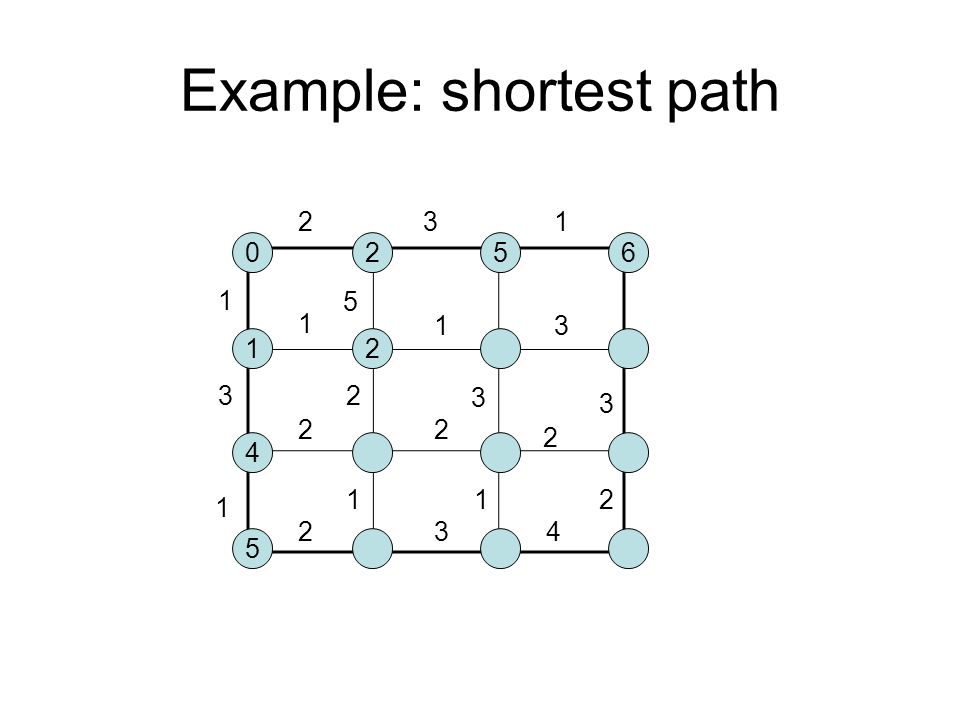
Example Find the shortest path in a grid s g 1 2 3 1 1 5 2 2 31 13 3 3 3 2 2 2 4 112 (0,0) (3,3)
 (3,3)")
13
Optimal substructure If a path P(s, g) is optimal, any sub-path, P(s,x), where x is on P(s,g), is also optimal Proof by contradiction –If the path between P(s,x) is not the shortest, i.e., P’(s,x) < P(s,x) –Construct a new path P’(s,g) = P’(s,x) + P(x, g) –P’(s,g) P(s,g) is not the shortest –Contradiction
 is optimal, any sub-path, P(s,x), where x is on P(s,g), is also optimal Proof by contradiction –If the path between P(s,x) is not the shortest, i.e., P’(s,x) < P(s,x) –Construct a new path P’(s,g) = P’(s,x) + P(x, g) –P’(s,g) P(s,g) is not the shortest –Contradiction")
14
Overlapping sub-problems Some sub-problems are used by many paths (0,0) -> (2,0) used by 3 paths
 -> (2,0) used by 3 paths")
15
Memorization and reuse Easy to tabulate and reuse –Number of sub-problems ~ number of nodes –P(s, x), for x in all nodes except s and g Find an order such that no sub-problems need to be recomputed –First compute the smallest sub-problems –Use solutions of small sub-problems to solve large sub-problems
, for x in all nodes except s and g Find an order such that no sub-problems need to be recomputed –First compute the smallest sub-problems –Use solutions of small sub-problems to solve large sub-problems")
16
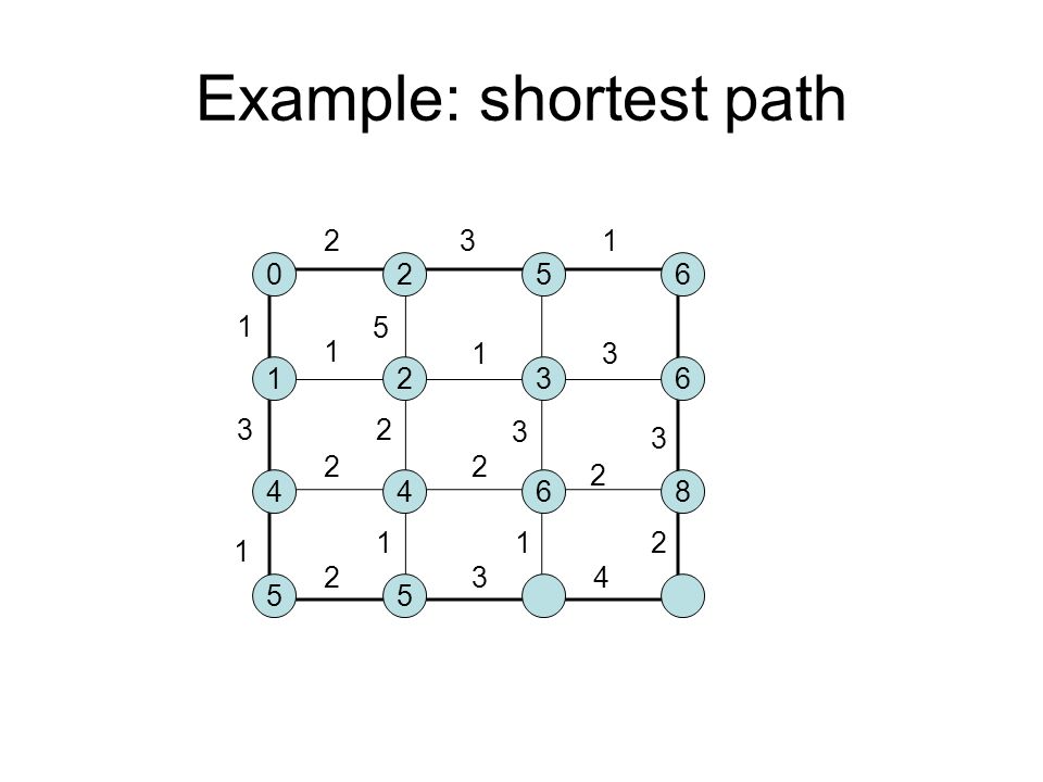
0 1 2 3 1 1 5 2 2 31 13 3 3 3 2 2 2 4 112 Example: shortest path

17
02 1 56 4 5 1 2 3 1 1 5 2 2 31 13 3 3 3 2 2 2 4 112

18
02 1 56 2 4 5 1 2 3 1 1 5 2 2 31 13 3 3 3 2 2 2 4 112
19
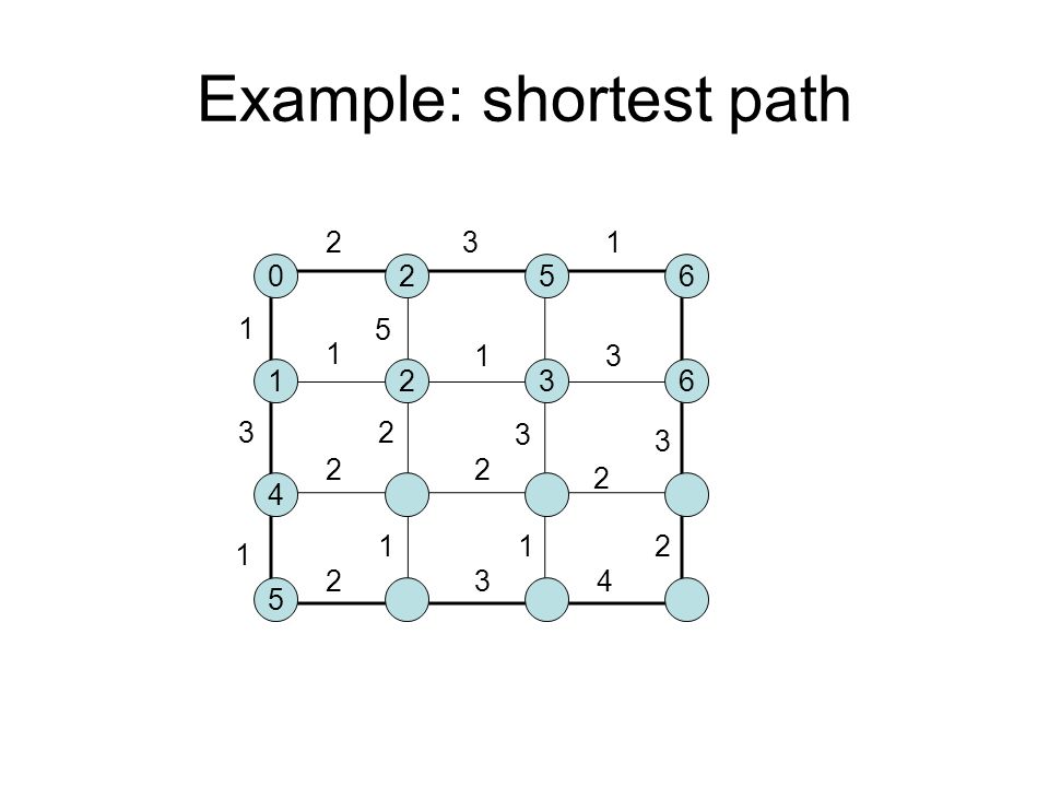
02 1 56 23 4 5 1 2 3 1 1 5 2 2 31 13 3 3 3 2 2 2 4 112

20
02 1 56 236 4 5 1 2 3 1 1 5 2 2 31 13 3 3 3 2 2 2 4 112
21
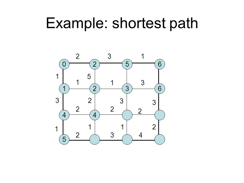
02 1 56 236 44 5 1 2 3 1 1 5 2 2 31 13 3 3 3 2 2 2 4 112
22
02 1 56 236 446 5 1 2 3 1 1 5 2 2 31 13 3 3 3 2 2 2 4 112

23
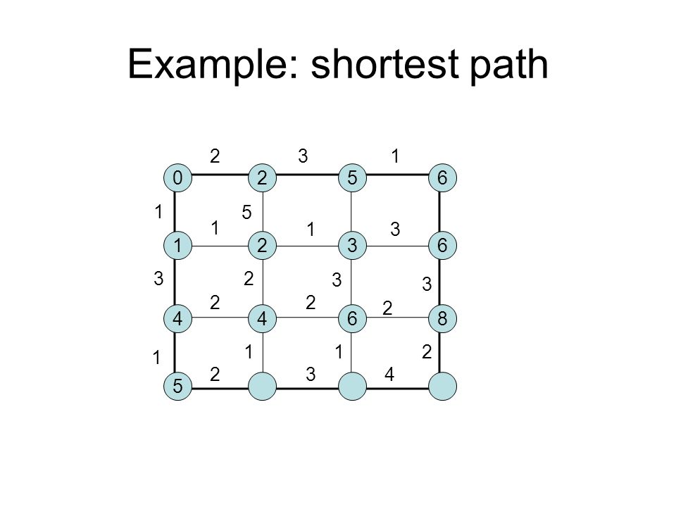
02 1 56 236 4468 5 1 2 3 1 1 5 2 2 31 13 3 3 3 2 2 2 4 112
24
02 1 56 236 4468 55 1 2 3 1 1 5 2 2 31 13 3 3 3 2 2 2 4 112
25
02 1 56 236 4468 557 1 2 3 1 1 5 2 2 31 13 3 3 3 2 2 2 4 112

26
02 1 56 236 4468 55710 1 2 3 1 1 5 2 2 31 13 3 3 3 2 2 2 4 112 Example: shortest path

27
02 1 56 236 4468 55710 1 2 3 1 1 5 2 2 31 13 3 3 3 2 2 2 4 112 Example: shortest path

28
Analysis For a nxn grid Enumeration: –number of paths = (2n!)/(n!)^2 –Each path has 2n steps –Total operation: 2n * (2n!) / (n!)^2 = O(2^(2n)) Recursive call: O(2^(2n)) DP: O(n^2)
/(n!)^2 –Each path has 2n steps –Total operation: 2n * (2n!) / (n!)^2 = O(2^(2n)) Recursive call: O(2^(2n)) DP: O(n^2)")
29
EnumerationRecursionDP N=31206824 N=52,5201,03260 N=103,695,1201,048,576420

30
Example: Fibonacci Seq F(n) = F(n-1) + F(n-2), F(0) = F(1) = 1 Function fib(n) if (n == 0 or n == 1) return 1; else return fib(n-1) + fib(n-2);
 = F(n-1) + F(n-2), F(0) = F(1) = 1 Function fib(n) if (n == 0 or n == 1) return 1; else return fib(n-1) + fib(n-2);")
31
Time complexity: O(1.62^n)
")
32
Example: Fibonacci Seq function fib(n) F[0] = 1;F[1] = 1; For i = 2 to n F[n] = F[n-1] + F[n-2]; End Return F[n];
![Example: Fibonacci Seq function fib(n) F[0] = 1;F[1] = 1; For i = 2 to n F[n] = F[n-1] + F[n-2]; End Return F[n];](http://images.slideplayer.com/32/9899056/slides/slide_32.jpg "Example: Fibonacci Seq function fib(n) F[0] = 1;F[1] = 1; For i = 2 to n F[n] = F[n-1] + F[n-2]; End Return F[n];")
33
11235813213455 Time: O(n), space: O(n)
, space: O(n)")
34
What if it is not so easy to figure out an order to fill in the table? Exercise

35
Today’s lecture Sequence alignment –Global alignment

36
Why seq alignment? Similar sequences often have similar origin or function –Two genes are said to be homologous if they share a common evolutionary history. –Evolutionary history can tell us a lot about properties of a given gene –Homology can be inferred from similarity between the genes New protein sequences are always compared to sequence databases to search for proteins with same or similar functions Most widely used computational tools in biology

37
Evolution at the DNA level …ACGGTGCAGTCACCA… …ACGTTGC-GTCCACCA… C Sequence edits: Mutation, deletion, insertion

38
Evolutionary Rates OK X X Still OK? next generation

39
Sequence conservation implies function

40
Sequence Alignment -AGGCTATCACCTGACCTCCAGGCCGA--TGCCC--- TAG-CTATCAC--GACCGC--GGTCGATTTGCCCGAC Definition An alignment of two string S, T is a pair of strings S ’, T ’ (with spaces) s.t. (1) |S ’ | = |T ’ |, and (|S| = “ length of S ” ) (2) removing all spaces in S ’, T ’ leaves S, T AGGCTATCACCTGACCTCCAGGCCGATGCCC TAGCTATCACGACCGCGGTCGATTTGCCCGAC
 |S ’ | = |T ’ |, and (|S| = length of S ) (2) removing all spaces in S ’, T ’ leaves S, T AGGCTATCACCTGACCTCCAGGCCGATGCCC TAGCTATCACGACCGCGGTCGATTTGCCCGAC.")
41
What is a good alignment? Alignment: The “ best ” way to match the letters of one sequence with those of the other How do we define “ best ” ?

42
The score of aligning (characters or spaces) x & y is σ (x,y). Score of an alignment: An optimal alignment: one with max score S’: -AGGCTATCACCTGACCTCCAGGCCGA--TGCCC--- T’: TAG-CTATCAC--GACCGC--GGTCGATTTGCCCGAC

43
Scoring Function Sequence edits: AGGCCTC –Mutations AGGACTC –InsertionsAGGGCCTC –DeletionsAGG-CTC Scoring Function: Match: +m~~~AAC~~~ Mismatch: -s~~~A-A~~~ Gap (indel):-d
:-d")
44
More complex scoring function Substitution matrix –Similarity score of matching two letters a, b should reflect the probability of a, b derived from same ancestor –It is usually defined by log likelihood ratio (Durbin book) –Active research area. Especially for proteins. –Commonly used: PAM, BLOSUM

45
An example substitution matrix ACGT A3-2-2 C3 G3-2 T3

46
Match = 2, mismatch = -1, gap = -1 Score = 3 x 2 – 2 x 1 – 1 x 1 = 3

47
How to find it? A naïve algorithm: for all subseqs A of S, B of T s.t. |A| = |B| do align A[i] with B[i], 1 ≤i ≤|A| align all other chars to spaces compute its value retain the max end output the retained alignment S = abcd A = cd T = wxyz B = xz -abc-d a-bc-d w--xyz -w-xyz

48
Analysis Assume |S| = |T| = n Cost of evaluating one alignment: ≥n How many alignments are there: –pick n chars of S,T together –say k of them are in S –match these k to the k unpicked chars of T Total time: E.g., for n = 20, time is > 2 40 >10 12 operations

49
Dynamic Programming We will now describe a dynamic programming algorithm Suppose we wish to align x 1 ……x M y 1 ……y N Let F(i,j) = optimal score of aligning x 1 ……x i y 1 ……y j
 = optimal score of aligning x 1 ……x i y 1 ……y j")
50
Dynamic Programming (cont ’ d) Notice three possible cases: 1.x M aligns to y N ~~~~~~~ x M ~~~~~~~ y N 2.x M aligns to a gap ~~~~~~~ x M ~~~~~~~ - 3.y N aligns to a gap ~~~~~~~ - ~~~~~~~ y N m, if x M = y N F(M,N) = F(M-1, N-1) + -s, if not F(M,N) = F(M-1, N) - d F(M,N) = F(M, N-1) - d
 Notice three possible cases: 1.x M aligns to y N ~~~~~~~ x M ~~~~~~~ y N 2.x M aligns to a gap ~~~~~~~ x M ~~~~~~~ - 3.y N aligns to a gap ~~~~~~~ - ~~~~~~~ y N m, if x M = y N F(M,N) = F(M-1, N-1) + -s, if not F(M,N) = F(M-1, N) - d F(M,N) = F(M, N-1) - d")
51
Therefore: F(M-1, N-1) + (X M,Y N ) F(M,N) = max F(M-1, N) – d F(M, N-1) – d (X M,Y N ) = m if X M = Y N, and –s otherwise Each sub-problem can be solved recursively
 + (X M,Y N ) F(M,N) = max F(M-1, N) – d F(M, N-1) – d (X M,Y N ) = m if X M = Y N, and –s otherwise Each sub-problem can be solved recursively")
52
Generalize: F(i-1, j-1) + (X i,Y j ) F(i,j) = max F(i-1, j) – d F(i, j-1) – d Be careful with the boundary conditions
 + (X i,Y j ) F(i,j) = max F(i-1, j) – d F(i, j-1) – d Be careful with the boundary conditions")
53
Remember: –The recursive formula is for understanding the relationship between sub-problems –We cannot afford to really solve them recursively Number of sub-problems: –Each corresponds to calculating an F(i, j) –O(MN) of them –Solve all of them
 –O(MN) of them –Solve all of them")
54
What order to fill? F(0,0) F(M,N)
 F(M,N)")
55
F(i-1, j-1) + (X i,Y j ) F(i, j) = max F(i-1, j) – d F(i, j-1) – d F(i, j)F(i, j-1) F(i-1, j)F(i-1, j-1) [case 1] [case 2] [case 3] 1 2 3
![F(i-1, j-1) + (X i,Y j ) F(i, j) = max F(i-1, j) – d F(i, j-1) – d F(i, j)F(i, j-1) F(i-1, j)F(i-1, j-1) [case 1] [case 2] [case 3] 1 2 3](http://images.slideplayer.com/32/9899056/slides/slide_55.jpg "F(i-1, j-1) + (X i,Y j ) F(i, j) = max F(i-1, j) – d F(i, j-1) – d F(i, j)F(i, j-1) F(i-1, j)F(i-1, j-1) [case 1] [case 2] [case 3] 1 2 3")
56
What order to fill? F(0,0) F(M,N)
 F(M,N)")
57
Example x = AGTAm = 1 y = ATAs = -1 d = -1 AGTA A T A F(i,j) i = 0 1 2 3 4 j = 0 1 2 3
 i = j =")
58
Example x = AGTAm = 1 y = ATAs = -1 d = -1 AGTA 0-2-3-4 A T-2 A-3 j = 0 1 2 3 F(i,j) i = 0 1 2 3 4
 i =")
59
Example x = AGTAm = 1 y = ATAs = -1 d = -1 AGTA 0-2-3-4 A10 -2 T A-3 j = 0 1 2 3 F(i,j) i = 0 1 2 3 4
 i =")
60
Example x = AGTAm = 1 y = ATAs = -1 d = -1 AGTA 0-2-3-4 A10 -2 T 0010 A-3 j = 0 1 2 3 F(i,j) i = 0 1 2 3 4
 i =")
61
Example x = AGTAm = 1 y = ATAs = -1 d = -1 AGTA 0-2-3-4 A10 -2 T 0010 A-3 02 j = 0 1 2 3 Optimal Alignment: F(4,3) = 2 F(i,j) i = 0 1 2 3 4
 = 2 F(i,j) i =")
62
Example x = AGTAm = 1 y = ATAs = -1 d = -1 AGTA 0-2-3-4 A10 -2 T 0010 A-3 02 j = 0 1 2 3 Optimal Alignment: F(4,3) = 2 This only tells us the best score F(i,j) i = 0 1 2 3 4
 = 2 This only tells us the best score F(i,j) i =")
63
Trace-back x = AGTAm = 1 y = ATAs = -1 d = -1 AGTA 0-2-3-4 A10 -2 T 0010 A-3 02 j = 0 1 2 3 F(i-1, j-1) + (Xi,Yj) F(i,j) = max F(i-1, j) – d F(i, j-1) – d F(i,j) i = 0 1 2 3 4
 + (Xi,Yj) F(i,j) = max F(i-1, j) – d F(i, j-1) – d F(i,j) i =")
64
Trace-back AGTA 0-2-3-4 A10 -2 T 0010 A-3 02 F(i-1, j-1) + (Xi,Yj) F(i,j) = max F(i-1, j) – d F(i, j-1) – d x = AGTAm = 1 y = ATAs = -1 d = -1 j = 0 1 2 3 F(i,j) i = 0 1 2 3 4
 + (Xi,Yj) F(i,j) = max F(i-1, j) – d F(i, j-1) – d x = AGTAm = 1 y = ATAs = -1 d = -1 j = F(i,j) i =")
65
Trace-back x = AGTAm = 1 y = ATAs = -1 d = -1 AGTA 0-2-3-4 A10 -2 T 0010 A-3 02 j = 0 1 2 3 F(i-1, j-1) + (Xi,Yj) F(i,j) = max F(i-1, j) – d F(i, j-1) – d F(i,j) i = 0 1 2 3 4
 + (Xi,Yj) F(i,j) = max F(i-1, j) – d F(i, j-1) – d F(i,j) i =")
66
Trace-back x = AGTAm = 1 y = ATAs = -1 d = -1 AGTA 0-2-3-4 A10 -2 T 0010 A-3 02 j = 0 1 2 3 F(i-1, j-1) + (Xi,Yj) F(i,j) = max F(i-1, j) – d F(i, j-1) – d F(i,j) i = 0 1 2 3 4
 + (Xi,Yj) F(i,j) = max F(i-1, j) – d F(i, j-1) – d F(i,j) i =")
67
Trace-back x = AGTAm = 1 y = ATAs = -1 d = -1 AGTA 0-2-3-4 A10 -2 T 0010 A-3 02 j = 0 1 2 3 Optimal Alignment: F(4,3) = 2 AGTA A TA F(i-1, j-1) + (Xi,Yj) F(i,j) = max F(i-1, j) – d F(i, j-1) – d F(i,j) i = 0 1 2 3 4
 = 2 AGTA A TA F(i-1, j-1) + (Xi,Yj) F(i,j) = max F(i-1, j) – d F(i, j-1) – d F(i,j) i =")
68
In some cases, trace-back may be very time consuming Alternative solution: remember where you come from! –Trade-off: more memory

69
Using trace-back pointers x = AGTAm = 1 y = ATAs = -1 d = -1 AGTA 0-2-3-4 A T-2 A-3 j = 0 1 2 3 F(i,j) i = 0 1 2 3 4
 i =")
70
Using trace-back pointers x = AGTAm = 1 y = ATAs = -1 d = -1 AGTA 0-2-3-4 A10 -2 T A-3 j = 0 1 2 3 F(i,j) i = 0 1 2 3 4
 i =")
71
Using trace-back pointers x = AGTAm = 1 y = ATAs = -1 d = -1 AGTA 0-2-3-4 A10 -2 T 0010 A-3 j = 0 1 2 3 F(i,j) i = 0 1 2 3 4
 i =")
72
Using trace-back pointers x = AGTAm = 1 y = ATAs = -1 d = -1 AGTA 0-2-3-4 A10 -2 T 0010 A-3 02 j = 0 1 2 3 F(i,j) i = 0 1 2 3 4
 i =")
73
Using trace-back pointers x = AGTAm = 1 y = ATAs = -1 d = -1 AGTA 0-2-3-4 A10 -2 T 0010 A-3 02 j = 0 1 2 3 F(i,j) i = 0 1 2 3 4
 i =")
74
Using trace-back pointers x = AGTAm = 1 y = ATAs = -1 d = -1 AGTA 0-2-3-4 A10 -2 T 0010 A-3 02 j = 0 1 2 3 F(i,j) i = 0 1 2 3 4
 i =")
75
Using trace-back pointers x = AGTAm = 1 y = ATAs = -1 d = -1 AGTA 0-2-3-4 A10 -2 T 0010 A-3 02 j = 0 1 2 3 F(i,j) i = 0 1 2 3 4
 i =")
76
Using trace-back pointers x = AGTAm = 1 y = ATAs = -1 d = -1 AGTA 0-2-3-4 A10 -2 T 0010 A-3 02 j = 0 1 2 3 Optimal Alignment: F(4,3) = 2 AGTA A TA F(i,j) i = 0 1 2 3 4
 = 2 AGTA A TA F(i,j) i =")
77
The Needleman-Wunsch Algorithm 1.Initialization. a.F(0, 0) = 0 b.F(0, j) = - j d c.F(i, 0)= - i d 2.Main Iteration. Filling in scores a.For each i = 1……M For each j = 1……N F(i-1,j) – d [case 1] F(i, j) = max F(i, j-1) – d [case 2] F(i-1, j-1) + σ(x i, y j ) [case 3] UP, if [case 1] Ptr(i,j)= LEFTif [case 2] DIAGif [case 3] 3.Termination. F(M, N) is the optimal score, and from Ptr(M, N) can trace back optimal alignment
 = 0 b.F(0, j) = - j d c.F(i, 0)= - i d 2.Main Iteration. Filling in scores a.For each i = 1……M For each j = 1……N F(i-1,j) – d [case 1] F(i, j) = max F(i, j-1) – d [case 2] F(i-1, j-1) + σ(x i, y j ) [case 3] UP, if [case 1] Ptr(i,j)= LEFTif [case 2] DIAGif [case 3] 3.Termination. F(M, N) is the optimal score, and from Ptr(M, N) can trace back optimal alignment.")
78
Performance Time: O(NM) Space: O(NM) Later we will cover more efficient methods
 Space: O(NM) Later we will cover more efficient methods")
79
A variant of the basic algorithm: Maybe it is OK to have an unlimited # of gaps in the beginning and end: ----------CTATCACCTGACCTCCAGGCCGATGCCCCTTCCGGC GCGAGTTCATCTATCAC--GACCGC--GGTCG-------------- Then, we don ’ t want to penalize gaps in the ends

80
The Overlap Detection variant Changes: 1.Initialization For all i, j, F(i, 0) = 0 F(0, j) = 0 2.Termination max i F(i, N) F OPT = max max j F(M, j) x 1 ……………………………… x M y N ……………………………… y 1
 = 0 F(0, j) = 0 2.Termination max i F(i, N) F OPT = max max j F(M, j) x 1 ……………………………… x M y N ……………………………… y 1")
81
Different types of overlaps x y x y

82
A non-bio variant Shell command “diff” in unix –Given file1 and file2 –Find the difference between file1 and file2 –Similar to sequence alignment –How to score? Longest common subsequence (LCS) Match has score 1 No mismatch penalty No gap penalty
 Match has score 1 No mismatch penalty No gap penalty.")
83
File1 A B C D E F File2 G B C E F

84
File1 A B C D E F File2 G B C - E F $ diff file1 file2 1c1 < A --- > G 4c4 < D --- > - LCS = 4

85
The LCS variant Changes: 1.Initialization For all i, j, F(i, 0) = F(0, j) = 0 2.Filling in table F(i-1,j) F(i, j) = max F(i, j-1) F(i-1, j-1) + σ(x i, y j ) where σ(x i, y j ) = 1 if x i = y j and 0 otherwise. 3.Termination max i F(i, N) F OPT = max max j F(M, j)
 F OPT = max max j F(M, j).")
86
What happens if you have 1 million lines of text in each file? Slow –What if the majority of the two files are the same? (e.g., two versions of a software) –Bounded DP Memory inefficient –At least 1000 GB memory –Linear-space algorithm, same time complexity
 –Bounded DP Memory inefficient –At least 1000 GB memory –Linear-space algorithm, same time complexity.")
87
See you next week

Similar presentations


*>")


