Download presentation
Presentation is loading. Please wait.

1
Indexing Structures Database System Implementation CSE 507 Some slides adapted from R. Elmasri and S. Navathe, Fundamentals of Database Systems, Sixth Edition, Pearson. And Silberschatz, Korth and Sudarshan Database System Concepts – 6 th Edition.

2
Indexes as Access Paths The index is usually specified on one field of the file (although it could be specified on several fields) One form of an index is a file of entries, which is ordered by field value The index is called an access path on the field. The index file is always ordered on the “indexing field value”

3
Indexes as Access Paths Contd The index file usually occupies considerably less disk blocks than the data file because its entries are much smaller A binary search on the index yields a pointer to the file record Indexes can also be characterized as dense or sparse A dense index has an index entry for every search key value (and hence every record) in the data file. A sparse (or nondense) index, on the other hand, has index entries for only some of the search values
 index, on the other hand, has index entries for only some of the search values.")
4
Single-Level Indexes Primary Index Defined on an ordered data file The data file is ordered on a key field Includes one index entry for each block in the data file; the index entry has the key field value for the first record in the block, which is called the block anchor A similar scheme can use the last record in a block. A primary index is a nondense (sparse) index. These are basically one level indirections. All records in the index file directly point to data.
 index. These are basically one level indirections. All records in the index file directly point to data..")
5
Sample Primary Index

6
Pop Question We have an ordered file with r = 30000 records stored on a disk with block size B = 1024 bytes. File records are of fixed size and are unspanned, with record length R = 100 bytes. What is the blocking factor of the file? Number of blocks needed for the file? Cost of Binary search? Ordering field = 9 bytes. Block pointer = 6 bytes. Blocking factor of the index? Number of blocks for the index file? Cost of binary search on the index file?

7
Pop Question -- Answers We have an ordered file with r = 30000 records stored on a disk with block size B = 1024 bytes. File records are of fixed size and are unspanned, with record length R = 100 bytes. What is the blocking factor of the file? Floor(1024/100) = 10 rec/block Number of blocks needed for the file? Ceil(30000/10) = 3000 blocks Cost of Binary search? Ceil(log 2 3000) = 12 Ordering field = 9 bytes. Block pointer = 6 bytes. Blocking factor of the index? Floor(1024/15) = 68 entries/blo Number of blocks for the index file? Ceil(3000/68) = 45 blocks Cost of binary search on the index file? Ceil(log 2 45) = 6
 = 10 rec/block Number of blocks needed for the file. Ceil(30000/10) = 3000 blocks Cost of Binary search. Ceil(log ) = 12 Ordering field = 9 bytes. Block pointer = 6 bytes. Blocking factor of the index. Floor(1024/15) = 68 entries/blo Number of blocks for the index file. Ceil(3000/68) = 45 blocks Cost of binary search on the index file. Ceil(log 2 45) = 6.")
8
Single-Level Indexes Clustering Index Defined on an ordered data file The data file is ordered on a non-key field unlike primary index. Includes one index entry for each distinct value of the field. the index entry points to the first data block that contains records with that field value. It is another example of nondense index.

9
Sample Clustering Index

10
Single-Level Indexes Secondary Index It is an alternative means of accessing (other than primary index). Can be created on any file organization (ordered, unordered or hashed). Can be created on any field, key (unique values) or non-key (duplicate values). Many secondary indexes can be created for a file. Only one primary index possible for a file. May have to be a dense index as data file records not ordered in indexing field.
. Can be created on any field, key (unique values) or non-key (duplicate values). Many secondary indexes can be created for a file. Only one primary index possible for a file. May have to be a dense index as data file records not ordered in indexing field..")
11
Sample Secondary Index --on Key Field Index Field ValueBlock pointer 1 2 3 6 8 10 12 13 12 6 1 3 8 10 2 14 Indexing Field (Secondary Key) …….
 …….")
12
Sample Secondary Index --on NonKey Index Field ValueBlock pointer 1 2 3 6 8 10 12 13 12 6 2 3 8 10 2 14 Indexing Field (Secondary Key) ……. Blocks of Record pointers

13
Pop Question We have an ordered file with r = 30000 records stored on a disk with block size B = 1024 bytes. File records are of fixed size and are unspanned, with record length R = 100 bytes. What is the blocking factor of the file? ---- 10 Number of blocks needed for the file? --- 3000 Cost of search on the non-ordering key? Index field = 9 bytes. Block pointer = 6 bytes. Blocking factor of the a secondary index? Number of blocks for the index file? Cost of binary search on the index file?

14
Pop Question We have an ordered file with r = 30000 records stored on a disk with block size B = 1024 bytes. File records are of fixed size and are unspanned, with record length R = 100 bytes. What is the blocking factor of the file? ---- 10 Number of blocks needed for the file? --- 3000 Cost of search on the non-ordering key? b/2 = 3000/2 = 1500 Index field = 9 bytes. Block pointer = 6 bytes. Blocking factor of the a secondary index? Will still be the same Floor(1024/15) Number of blocks for the index file? Ceil(30000/68) = 442 Cost of binary search on the index file? Ceil(Log 2 442) = 9
 Number of blocks for the index file. Ceil(30000/68) = 442 Cost of binary search on the index file. Ceil(Log 2 442) = 9.")
15
Summary of Single-Level Indexes

16
Multi-Level Indexes Since a single-level index is an ordered file, we can create a primary index to the index itself; The original index file is called the first-level index and the index to the index is called the second-level index. Can repeat to create a third, fourth,..., until all entries fit in one disk block A multi-level index can be created for any type of first-level index (primary, secondary, clustering) as long as the first-level index consists of more than one disk block
 as long as the first-level index consists of more than one disk block.")
17
A two level Primary Index

18
Constructing a Multi-Level Index Fan-out ( fo ) factor index blocking factor Divides the search space into n-ways (n == fan-out factor) Now searching in a multi-level index takes Log fo indexblocks Significantly smaller than the cost of binary search.
 factor index blocking factor Divides the search space into n-ways (n == fan-out factor) Now searching in a multi-level index takes Log fo indexblocks Significantly smaller than the cost of binary search.")
19
Constructing a Multi-Level Index If the first level contains r1 entries. Fanout fo = index blocking factor First needs Ceil(r1/ fo ) blocks. #index entries for second level r2 = Ceil(r1/ fo ) #index entries for third level r3 = Ceil(r2/ fo ) ……. Continues until all the entries of the index level not fit in a block. Approximately #levels = Ceil(Log fo r1)
 blocks. #index entries for second level r2 = Ceil(r1/ fo ) #index entries for third level r3 = Ceil(r2/ fo ) ……. Continues until all the entries of the index level not fit in a block. Approximately #levels = Ceil(Log fo r1).")
20
Pop Question We have an ordered file with r = 30000 records stored on a disk with block size B = 1024 bytes. File records are of fixed size and are unspanned, with record length R = 100 bytes. What is the blocking factor of the file? ---- 10 Number of blocks needed for the file? --- 3000 Cost of search on the non-ordering key? b/2 = 3000/2 = 1500 Index field = 9 bytes. Block pointer = 6 bytes. Blocking factor of the a secondary index? Will still be the same Floor(1024/15) Number of blocks for the index file? Ceil(30000/68) = 442 How many levels for a multi-level index?
 Number of blocks for the index file. Ceil(30000/68) = 442 How many levels for a multi-level index .")
21
Dynamic Multi-level Indexing

22
B+ -Tree The index file is organized as a B+ tree Height-balanced Nodes are blocks of index keys and pointers Order P: Max # of pointers fits in a node Nodes are at least 50% full Support efficient updates

23
B+ -Tree P = 4 100 120 150 180 30 3 5 30 31 35 100 101 110 120 122 130 150 151 156 180 182 200 Point to data records/blocks Index file Material adapted from Dr John Ortiz

24
B+ -Tree- Internal nodes Material adapted from Dr John Ortiz The root must have k 2 pointers Others must have k P/2 pointers, where P is the order of the B+ tree Root is an exception. Must have k keys and k+1 pointers Keys are sorted key >= a k … p0p0 a1a1 aiai pipi a i+1 pkpk ……akak a i <= key < a i+1 … key < a 1

25
B+ -Tree- Leaf nodes Material adapted from Dr John Ortiz to next Leaf node to data records a1a1 pr 1 aiai pr i NL pr k ……akak

26
A B+ -Tree Node

27
Searching in B+ -Tree Searching just like in a binary search tree Starts at the root, works down to the leaf level Does a comparison of the search value and the current “separation value”, goes left or right

28
Inserting in a B+ -Tree A search is first performed, using the value to be added After the search is completed, the location for the new value is known

29
Inserting in a B+ -Tree If the tree is empty, add to the root Once the root is full, split the data into 2 leaves, using the root to hold keys and pointers If adding an element will overload a leaf, take the median and split it

30
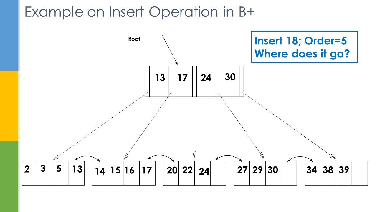
Example on Insert Operation in B+ Root 17 24 30 2 35 13 14 1620 22 24 272930343839 13 Insert 18; Order=5 Where does it go? 17 15
31
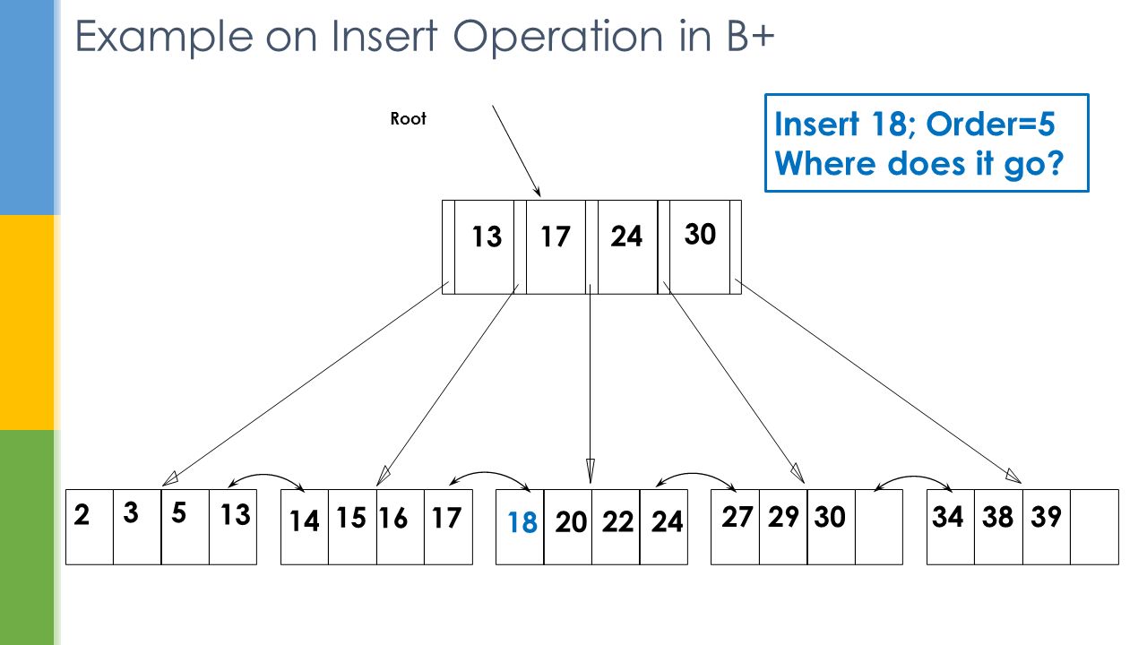
Example on Insert Operation in B+ Root 17 24 30 2 35 13 14 16 20 2224 272930343839 13 Insert 18; Order=5 Where does it go? 17 15 18
32
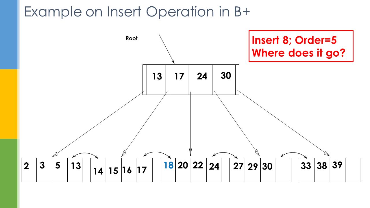
Example on Insert Operation in B+ Root 17 24 30 2 35 13 14 16 1820 22 27 29 33 38 39 13 Insert 8; Order=5 Where does it go? 17 2430 15
33
Example on Insert Operation in B+ Root 17 24 30 2 35 1314 16 20 22 27 29 33 38 39 13 Insert 8; Order=5 Where does it go? 172430 Leaf already full; Need to split 18 15

34
Example on Insert Operation in B+ Root 17 24 30 23 5 13 14 16 1820 22 24 27 29 33 30 38 39 13 Split along the median 8 New Leaf Insert 8; Order=5 17 15

35
Example on Insert Operation in B+ Root 17 24 30 2 35 13 14 16 20 22 24 27 29 33 30 38 39 13 8 New Leaf Insert 8; Order=5 17 18 Send the Median (5) to level above 15
 to level above 15")
36
Example on Insert Operation in B+ Root 17 24 30 2 3 5 13 14 1620 22 24 27 29 33 30 38 39 13 Send the Median (5) to level above 8 Insert 8; Order=5 17 18 15
 to level above 8 Insert 8; Order=")
37
Example on Insert Operation in B+ Root 17 24 30 2 3 5 13 14 16 20 22 24 27 29 33 30 38 39 13 8 Insert 8; Order=5 17 18 Send the Median (5) to level above; Also full; Need to split 15
 to level above; Also full; Need to split 15")
38
Example on Insert Operation in B+ Root 17 24 30 2 3 5 13 14 16 20 22 24 27 29 33 30 38 39 13 Split along the Median (17); Send Median a level above; New root! 8 Median (5) Added here Insert 8; Order=5 17 18 15
 Added here Insert 8; Order=")
39
Example on Insert Operation in B+ Root 13 2 3 5 14 16 20 22 24 27 29 33 30 38 39 5 Split along the Median (17); Send Median a level above; New root! 8 Insert 8; Order=5 1718 17 24 30 15

40
Example on Insert Operation in B+ 13 23 5 14 16 20 22 24 27 29 33 30 38 39 5 8 Insert 8; Order=5 17 18 17 24 30 17 is the new Root 15

41
Deletion in B+ -Tree Find the key to be deleted Remove (search-key value, pointer) from the leaf node If the node has too few entries (underflow) due to the removal We have two options: (a) Merge siblings or (b) Redistribution Material adapted from Silberchatz, Korth and Sudarshan
 from the leaf node If the node has too few entries (underflow) due to the removal We have two options: (a) Merge siblings or (b) Redistribution Material adapted from Silberchatz, Korth and Sudarshan")
42
Deletion in B+ -Tree – Merging Siblings Insert all the search-key values in the two nodes into a single node (the one on the left or right). Depending on left of right, the algorithm will vary slightly. Delete the other node. Delete the pair (K i–1, P i ), where P i is the pointer to the deleted node from its parent. Proceed to upper levels recursively as necessary. Material adapted from Silberchatz, Korth and Sudarshan
, where P i is the pointer to the deleted node from its parent. Proceed to upper levels recursively as necessary. Material adapted from Silberchatz, Korth and Sudarshan.")
43
Deletion in B+ -Tree – Redistribution Siblings After removal, the entries in the node and a sibling do not fit into a single node, then redistribute pointers : Redistribute the pointers between the node and a sibling such that both have more than the minimum number of entries. Update the corresponding search-key value in the parent of the node. Material adapted from Silberchatz, Korth and Sudarshan

44
Deletion in B+ -Tree Contd… The node deletions may cascade upwards till a node which has n/2 or more pointers is found. If the root node has only one pointer after deletion, it is deleted and the sole child becomes the root.

45
Example on Deletion operation in B+ -Tree 10 25 16 20 22 29 33 30 38 5 8 18 22 30 Order = 4 15 16

46
Example on Deletion operation in B+ -Tree 10 25 16 20 22 29 33 30 38 5 8 18 22 30 Delete 38 15 16

47
Example on Deletion operation in B+ -Tree 10 25 16 20 22 29 33 30 5 8 18 22 30 Delete 38 15 16 Underflow

48
Example on Deletion operation in B+ -Tree 10 25 16 20 22 29 33 30 5 8 18 22 30 Delete 38 15 16 Merging

49
Example on Deletion operation in B+ -Tree 10 25 16 20 22 29 33 30 5 8 18 22 30 Delete 38 15 16 Merging

50
Example on Deletion operation in B+ -Tree 10 25 16 20 22 29 33 30 5 8 18 22 30 Delete 38 15 16 Delete these

51
Example on Deletion operation in B+ -Tree 10 25 16 20 22 29 33 30 5 8 18 22 Delete 38 15 16 Underflow 30

52
Example on Deletion operation in B+ -Tree 10 25 16 20 22 29 33 30 5 8 18 22 Delete 38 15 16 Cannot merge with this node 30

53
Example on Deletion operation in B+ -Tree 10 25 16 20 22 29 33 30 5 8 18 22 Delete 38 15 16 Thus, we will re-distribute 30

54
Example on Deletion operation in B+ -Tree 10 25 16 20 22 29 33 30 5 8 18 22 Delete 38 15 16 16 is removed from here. It goes to root 30

55
Example on Deletion operation in B+ -Tree 10 25 16 20 22 29 33 30 5 8 18 22 Delete 38 15 16 22 from root Comes here along with pointer to leaf containing 18, 20, 22 30

56
Example on Deletion operation in B+ -Tree 10 25 16 20 22 29 33 30 5 8 18 22 Delete 38 15 Other pointers are shifted 16

57
Example on Deletion operation in B+ -Tree 10 25 16 20 22 29 33 30 5 8 18 22 Delete 33, 30 15 16

58
Example on Deletion operation in B+ -Tree 10 25 16 20 22 29 33 30 5 8 18 22 Delete 33, 30 15 16 No issues in deleting 33

59
Example on Deletion operation in B+ -Tree 10 25 16 20 22 29 30 5 8 18 22 Delete 30 15 16 Now this is underflow

60
Example on Deletion operation in B+ -Tree 10 25 16 20 22 29 5 8 18 22 Delete 30 15 16 Merge or Redistribute?

61
Example on Deletion operation in B+ -Tree 10 25 16 2022 29 5 8 18 22 Delete 30 15 16 22 moves here

62
Example on Deletion operation in B+ -Tree 10 25 16 2022 29 5 8 18 20 Final result after deleting 30 15 16 20 replaces 22 in the parent

63
Example on Deletion operation in B+ -Tree 10 25 16 2022 29 5 8 18 20 Delete 18 15 16

64
Example on Deletion operation in B+ -Tree 10 25 16 2022 29 5 8 18 20 Delete 18 15 16 Underflow, merge with sibling

65
Example on Deletion operation in B+ -Tree 10 25 16 20 22 29 5 8 20 Delete 18 15 16 Underflow, merge with sibling

66
Example on Deletion operation in B+ -Tree 10 25 16 20 22 29 5 8 20 Delete 18 15 16 Underflow, merge with sibling

67
Example on Deletion operation in B+ -Tree 10 25 16 20 22 29 5 8 16 Delete 18 15 16 Move pointers. And delete the root as it has only one child

68
Example on Deletion operation in B+ -Tree 10 25 16 20 22 29 5 8 16 Final result after deleting 18 15

69
Indexing Strings in B+ - Tree Variable length strings as keys Variable fanout Use space utilization as criterion for splitting, not number of pointers Prefix compression Key values at internal nodes can be prefixes of full key Keep enough characters to distinguish entries in the subtrees separated by the key value E.g. “Shailaja” and “Shailendra” can be separated by “Shaila” Keys in leaf node can be compressed by sharing common prefixes Material adapted from Silberchatz, Korth and Sudarshan

70
Bulk loading entries in B+ - Tree Inserting entries one-at-a-time into a B + -tree requires 1 IO per entry can be very inefficient for loading a large number of entries at a time ( bulk loading ) Efficient alternative 1: Sort entries first (using efficient external-memory algorithms) Insert in sorted order Insertion will go to existing page (or cause a split). Much improved IO performance. Material adapted from Silberchatz, Korth and Sudarshan

71
Bulk loading entries in B+ - Tree Efficient alternative 2: Bottom-up B + -tree construction As before sort entries And then create tree layer-by-layer, starting with leaf level. Implemented as part of bulk-load utility by most database systems Material adapted from Silberchatz, Korth and Sudarshan

72
Non-unique Search Queries in B+ - Tree Material adapted from Silberchatz, Korth and Sudarshan Store the key as many times as it appears. List of tuple pointers with each distinct value of key Extra code to handle long lists.

73
Difference between B-Tree and B+ - Tree In a B-tree, pointers to data records exist at all levels of the tree In a B+-tree, all pointers to data records exists at the leaf-level nodes

74
A B-Tree Node

75
B-Tree Vs B+ - Tree Material adapted from Silberchatz, Korth and Sudarshan Advantages of B-Tree indices: May use less tree nodes than a corresponding B + -Tree. Sometimes possible to find search-key value before reaching leaf node. Disadvantages of B-Tree indices: Only small fraction of all search-key values are found early Non-leaf nodes are larger, so fan-out is reduced. Thus, B-Trees typically have greater depth than corresponding B + -Tree A B+-tree can have less levels (or higher capacity of search values) than the corresponding B-tree Typically, advantages of B-Trees do not out weigh disadvantages.
 than the corresponding B-tree Typically, advantages of B-Trees do not out weigh disadvantages..")
Similar presentations


. Can make sense because records may be much.>")
. Can make sense because records may be much.>")


