1. Computer Performance Modeling Dirk Grunwald Prelude to Jain, Chapter 12 Laws of Large Numbers and The normal distribution

2. Weak Law of Large Numbers u Assume we conduct a random experiment n times, and let S n be the number of times that event A occurs. u We intuitively assume that u Let A be an event with probability P[A] and suppose we perform a Bernoulli sequence of n trials, where a success corresponds to an occurrence of event A. u S n has Binomial distribution with E[S n ]=nP[A] and Var[S n ]=nP[A](1-P[A])

3. Weak Law of Large Numbers u Thus, E[S n /n]=1/n E[S n ]=P[A] u Var[S n /n]=1/n 2 Var[S n ] = P[A](1-P[A]) / n u Now, apply Chebyshev’s inequality... u We can make the right hand side arbitrarily small by increasing n. u This shows that P[A] can be estimated from S n /n.

4. How large should n be? u If we apply Chebyshev’s inequality, u Clearly, p(1-p) has maximum at 1/2. Hence, no matter the value of p, we need to be certain

5. How large should n be? u If we know approximately what the value of p is, we see that this will be satisfied if or u If we have no idea what p is, then will be a (very) sloppy bound.

6. Applying the Weak Law u Assuming that each terminal in an interactive system has the same probability p of being in use during the peak period of the day. u We want to know how many observations n need to be made such that u In other words, we want to know that we’ve approximated p within 0.1 with reasonable (95%) confidence.

7. Applying the Weak Law u If the first 100 observations indicate that p is ~0.2, how many more trials are needed? u Using the sloppy bound… u But, knowing that p = ~0.2, we can use

8. The Weak Law & Central Limit u The weak law is a powerful tool, but it’s fairly imprecise. u We’re about to look at the Central Limit Theorem, which show us that 62 samples would be enough to estimate p. u To understand the central limit theorem, we need to visit the normal distribution.

9. Normal Distribution u A continuous random variable X is normal with parameters  and  >0 if it has the density function u We indicate this by writing X~N( ,  2 ). u A standard normal is N(0,1), where the standarrd normal density is

10. Standard Normal Distribution u The corresponding standard normal distribution function is therefore: u The standard normal is important, because you can calculate every normal using it. u If X~N( ,  2 ),then u You look this up in the CRC, Stats books or in Mathematica

11. Properties of Normal Distributions u Suppose X 1, X 2, …, X n are n independent R.V.’s such that X 1 ~ N(  1,  1 2 ), etc. Then, Y= X 1 + X 2 + …+ X n is normally distributed with mean  1+  2+…+  n and variance  1 2+  2 2+…+  n 2 u The normal distribution is symmetric around the mean: f(  +x)= f(  -x) u This symmetry is needed when looking up the standard normal in tables.

12. The Standard Normal ++-- 0.68268  -2  +2  Area under curve is 0.9545

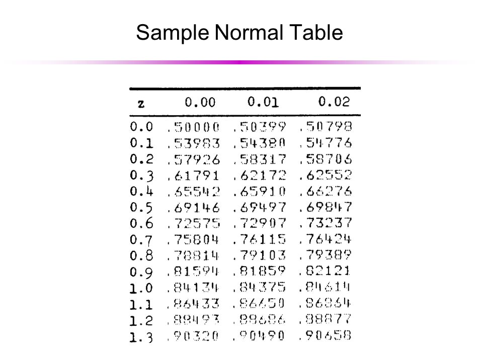
13. Sample Normal Table

15. Example: Normal Distribution u Suppose the number of buffers for a message system X~N(100,100). u Calculate the probability that the number of buffers in use does not exceed 120. Well, 120 is two standard deviations out. Thus, looking up N(0,1) for the value 2 is 0.97725. u What’s the probability it’s between 80 and 120 buffers? This is F(2)-F(-2) =.97725-(1-.97725), or 0.9545. u What’s P[X>=130]? This is 3 standard deviations out, tables show it’s 1-0.99865 or 0.00135.

16. Central Limit Theorem u Suppose X 1, X 2, …, X n are n identical independent R.V.’s with mean  and variance  2. Let S n = X 1 + X 2 + …+ X n. Then, for each x<y: u In other words, regardless of the underlying distribution, S n ~N( n , n  2 ) for some sufficiently large n.

17. But wait, it gets better! u The terms of S n don’t even have to have the same distribution, within some reasonable constraints. u This is the basis for the observation the sum of many random variables (height, IQ, grades in classes) tend to be normally distributed.

18. Limiting Samples using the Central Limit Theorem u Recall that a binomial distribution has mean np and variance npq, where q=(1-p). Now, consider an experiment where we determine if a sample obeys a property, and we want to determine P[A] from S n, much as in the Law of Weak Numbers. u We saw that allowed us to approximate the n needed to estimate that S n =p with some precision.

19. We can transform this into a something handled by the Central Limit Theorem

20. Applying the Central Limit Theorem u So, we can conclude.. u Or, that where..

21. Applying the Central Limit Theorem u Now, we look up the value of r that makes this equation hold. The definition of r now yields the following estimate for n. u The right hand side is because pq is maximal at p=1/2.

22. Example: Estimating Needed Samples u Same problem as earlier. Sample terminals 100 times, computer S n, and then assume that S n /n approximates p. u For  =0.05, we find that r=1.96 (using the normal tables). Using the previous equation, we find that n=96, assuming the approximate value of p=0.2. u However, this approximates p to the range 0.1..0.3. We can do better.

23. Example: Estimating Needed Samples u “If we make 500 observations to estimate p and let  =0.05, what is the value of  ?” u In other words, what is the maximum error in the estimate at the 5% level of uncertainty? u As before,  =0.05 implies r=1.96. u This has values in the range 0.0438..0.0351, depending on p.

24. So who cares? u The central limit theorem and the normal distribution will be combined to produce a powerful tool -- the confidence interval (see Jain, chapter 13). u This tool will be used to determine when l Observations are “statisically different” l We’ve know we’ve made enough observations in an experiment l We can placate thesis committees and bosses.

25. Quantiles -0.85 Area under graph is 0.20

26. Quantiles

27. Measures of Central Tendencies u Mean l Expectation for the distribution u Median l The Q50, or 50% quantile. l Half the samples have value less than this. u Mode l Most common value

28. Selecting the Right Central Metric

29. Detecting Skew

30. Harmonic Mean u Useful for analyzing benchmarks u “Suppose you drive your car one mile at 20 miles per hour and a second mile at 60 miles per hour. What is your average speed for the two miles?” l Not 40 MPH - we didn’t drive for equal times! l It took 3 minutes to drive first mile It took 1 minutes to drive second mile It took 4 minutes to drive a total of two miles u Therefore, average speed was 30 MPH

31. Harmonic Mean u If we define the harmonic mean to be... u Then, for our example, we get..

32. Harmonic Mean u Program A and B each require the 1,000,000 instructions on computer X. u Program A makes better use of caches, and executes at 2,000,000 inst/sec. (0.5 sec) u Program B only runs at 500,000 inst/sec (2sec) u What is the average instruction execution rate of program A and B?

33. Harmonic Mean u Harmonic mean should be used for summarizing performance expressed as a rate. It corresponds accurately with computation time that will actually be consumed by running real programs. Harmonic mean, when applied to a rate, is equivalent to calculating the total number of operations divided by the total time. u But, this only holds if the programs run for the same number of instructions, or the cars drive for the same distance at different speeds

34. Generalized (Weighted) Harmonic Mean u Suppose a sequence of programs of path lengths l 1, l 2, …, l n instructions run at the rates s 1, s 2, …., s n. u Then, the generalized harmonic mean is

35. Generalized Harmonic Mean u A company wants to measure the MIPS of one of their computers, based on the performance of three computers. Runs/DayInst/RunMIPS/Run f i l i S i 10303 20404 15305 u Use G.H.M with (f i *l i ) instructions, executed at rate S i. u Average MIPS is 3.974

36. Geometric Mean u The arithmetic mean is used if the sum of a quantity is of interest. The geometric mean is used if the product is of interest. u For example, l First level cache has 10% miss rate l Second level cache has 5% miss rate l You’d use the G.M. to compute the “average” miss rate.

37. Example of Geometric Mean u Given these improvements in different protocol layers: u Improvements in earlier layers influence performance of later layers. u Geometric mean of the improvements is 13%