Download presentation
Presentation is loading. Please wait.

1
Automatic Image Alignment with a lot of slides stolen from Steve Seitz and Rick Szeliski © Mike Nese CS194: Image Manipulation & Computational Photography Alexei Efros, UC Berkeley, Fall 2015

2
Live Homography DEMO Check out panoramio.com “Look Around” feature! Also see OpenPhoto VR: http://openphotovr.org/

3
Image Alignment How do we align two images automatically? Two broad approaches: Feature-based alignment –Find a few matching features in both images –compute alignment Direct (pixel-based) alignment –Search for alignment where most pixels agree
 alignment –Search for alignment where most pixels agree.")
4
Direct Alignment The simplest approach is a brute force search (hw1) Need to define image matching function –SSD, Normalized Correlation, edge matching, etc. Search over all parameters within a reasonable range: e.g. for translation: for tx=x0:step:x1, for ty=y0:step:y1, compare image1(x,y) to image2(x+tx,y+ty) end; Need to pick correct x0,x1 and step What happens if step is too large?
 to image2(x+tx,y+ty) end; Need to pick correct x0,x1 and step What happens if step is too large .")
5
Direct Alignment (brute force) What if we want to search for more complicated transformation, e.g. homography? for a=a0:astep:a1, for b=b0:bstep:b1, for c=c0:cstep:c1, for d=d0:dstep:d1, for e=e0:estep:e1, for f=f0:fstep:f1, for g=g0:gstep:g1, for h=h0:hstep:h1, compare image1 to H(image2) end; end; end; end;
 end; end; end; end;.")
6
Problems with brute force Not realistic Search in O(N 8 ) is problematic Not clear how to set starting/stopping value and step What can we do? Use pyramid search to limit starting/stopping/step values For special cases (rotational panoramas), can reduce search slightly to O(N 4 ): –H = K 1 R 1 R 2 -1 K 2 -1 (4 DOF: f and rotation) Alternative: gradient decent on the error function i.e. how do I tweak my current estimate to make the SSD error go down? Can do sub-pixel accuracy BIG assumption? –Images are already almost aligned (<2 pixels difference!) –Can improve with pyramid Same tool as in motion estimation
, can reduce search slightly to O(N 4 ): –H = K 1 R 1 R 2 -1 K 2 -1 (4 DOF: f and rotation) Alternative: gradient decent on the error function i.e. how do I tweak my current estimate to make the SSD error go down. Can do sub-pixel accuracy BIG assumption. –Images are already almost aligned (<2 pixels difference!) –Can improve with pyramid Same tool as in motion estimation.")
7
Image alignment

8
Feature-based alignment 1.Feature Detection: find a few important features (aka Interest Points) in each image separately 2.Feature Matching: match them across two images 3.Compute image transformation: as per Project #6 Part I How do we choose good features automatically? They must be prominent in both images Easy to localize Think how you did that by hand in Project #6 Part I Corners!

9
Feature Detection

10
Feature Matching How do we match the features between the images? Need a way to describe a region around each feature –e.g. image patch around each feature Use successful matches to estimate homography –Need to do something to get rid of outliers Issues: What if the image patches for several interest points look similar? –Make patch size bigger What if the image patches for the same feature look different due to scale, rotation, etc. –Need an invariant descriptor

11
Invariant Feature Descriptors Schmid & Mohr 1997, Lowe 1999, Baumberg 2000, Tuytelaars & Van Gool 2000, Mikolajczyk & Schmid 2001, Brown & Lowe 2002, Matas et. al. 2002, Schaffalitzky & Zisserman 2002

12
Today’s lecture 1 Feature detector scale invariant Harris corners 1 Feature descriptor patches, oriented patches Reading: Multi-image Matching using Multi-scale image patches, CVPR 2005

13
Invariant Local Features Image content is transformed into local feature coordinates that are invariant to translation, rotation, scale, and other imaging parameters Features Descriptors

14
Applications Feature points are used for: Image alignment (homography, fundamental matrix) 3D reconstruction Motion tracking Object recognition Indexing and database retrieval Robot navigation … other
 3D reconstruction Motion tracking Object recognition Indexing and database retrieval Robot navigation … other")
15
Feature Detector – Harris Corner

16
Harris corner detector C.Harris, M.Stephens. “A Combined Corner and Edge Detector”. 1988

17
The Basic Idea We should easily recognize the point by looking through a small window Shifting a window in any direction should give a large change in intensity

18
Harris Detector: Basic Idea “flat” region: no change in all directions “edge”: no change along the edge direction “corner”: significant change in all directions

19
Harris Detector: Mathematics Change of intensity for the shift [u,v]: Intensity Shifted intensity Window function or Window function w(x,y) = Gaussian1 in window, 0 outside
![Harris Detector: Mathematics Change of intensity for the shift [u,v]: Intensity Shifted intensity Window function or Window function w(x,y) = Gaussian1 in window, 0 outside](http://images.slideplayer.com/32/9843180/slides/slide_19.jpg "Harris Detector: Mathematics Change of intensity for the shift [u,v]: Intensity Shifted intensity Window function or Window function w(x,y) = Gaussian1 in window, 0 outside")
20
Harris Detector: Mathematics For small shifts [u,v ] we have a bilinear approximation: where M is a 2 2 matrix computed from image derivatives:
![Harris Detector: Mathematics For small shifts [u,v ] we have a bilinear approximation: where M is a 2 2 matrix computed from image derivatives:](http://images.slideplayer.com/32/9843180/slides/slide_20.jpg "Harris Detector: Mathematics For small shifts [u,v ] we have a bilinear approximation: where M is a 2 2 matrix computed from image derivatives:")
21
Harris Detector: Mathematics 1 2 “Corner” 1 and 2 are large, 1 ~ 2 ; E increases in all directions 1 and 2 are small; E is almost constant in all directions “Edge” 1 >> 2 “Edge” 2 >> 1 “Flat” region Classification of image points using eigenvalues of M:

22
Harris Detector: Mathematics Measure of corner response:

23
Harris Detector The Algorithm: Find points with large corner response function R (R > threshold) Take the points of local maxima of R
 Take the points of local maxima of R")
24
Harris Detector: Workflow

25
Compute corner response R

26
Harris Detector: Workflow Find points with large corner response: R>threshold

27
Harris Detector: Workflow Take only the points of local maxima of R

28
Harris Detector: Workflow

29
Harris Detector: Some Properties Rotation invariance Ellipse rotates but its shape (i.e. eigenvalues) remains the same Corner response R is invariant to image rotation
 remains the same Corner response R is invariant to image rotation.")
30
Harris Detector: Some Properties Partial invariance to affine intensity change Only derivatives are used => invariance to intensity shift I I + b Intensity scale: I a I R x (image coordinate) threshold R x (image coordinate)
 threshold R x (image coordinate)")
31
Harris Detector: Some Properties But: non-invariant to image scale! All points will be classified as edges Corner !

32
Scale Invariant Detection Consider regions (e.g. circles) of different sizes around a point Regions of corresponding sizes will look the same in both images
 of different sizes around a point Regions of corresponding sizes will look the same in both images.")
33
Scale Invariant Detection The problem: how do we choose corresponding circles independently in each image? Choose the scale of the “best” corner

34
Feature selection Distribute points evenly over the image

35
Adaptive Non-maximal Suppression Desired: Fixed # of features per image Want evenly distributed spatially… Sort points by non-maximal suppression radius [Brown, Szeliski, Winder, CVPR’05]
![Adaptive Non-maximal Suppression Desired: Fixed # of features per image Want evenly distributed spatially… Sort points by non-maximal suppression radius [Brown, Szeliski, Winder, CVPR’05]](http://images.slideplayer.com/32/9843180/slides/slide_35.jpg "Adaptive Non-maximal Suppression Desired: Fixed # of features per image Want evenly distributed spatially… Sort points by non-maximal suppression radius [Brown, Szeliski, Winder, CVPR’05]")
36
Feature descriptors We know how to detect points Next question: How to match them? ? Point descriptor should be: 1.Invariant2. Distinctive

37
Feature Descriptor – MOPS

38
Descriptors Invariant to Rotation Find local orientation Dominant direction of gradient Extract image patches relative to this orientation

39
Multi-Scale Oriented Patches Interest points Multi-scale Harris corners Orientation from blurred gradient Geometrically invariant to rotation Descriptor vector Bias/gain normalized sampling of local patch (8x8) Photometrically invariant to affine changes in intensity [Brown, Szeliski, Winder, CVPR’2005]
![Multi-Scale Oriented Patches Interest points Multi-scale Harris corners Orientation from blurred gradient Geometrically invariant to rotation Descriptor vector Bias/gain normalized sampling of local patch (8x8) Photometrically invariant to affine changes in intensity [Brown, Szeliski, Winder, CVPR’2005]](http://images.slideplayer.com/32/9843180/slides/slide_39.jpg "Multi-Scale Oriented Patches Interest points Multi-scale Harris corners Orientation from blurred gradient Geometrically invariant to rotation Descriptor vector Bias/gain normalized sampling of local patch (8x8) Photometrically invariant to affine changes in intensity [Brown, Szeliski, Winder, CVPR’2005]")
40
Detect Features, setup Frame Orientation = blurred gradient Rotation Invariant Frame Scale-space position (x, y, s) + orientation ( )
 + orientation ( )")
41
Detections at multiple scales

42
MOPS descriptor vector 8x8 oriented patch Sampled at 5 x scale Bias/gain normalisation: I’ = (I – )/ 8 pixels 40 pixels
/ 8 pixels 40 pixels")
43
Automatic Feature Matching

44
Feature matching ?

45
Pick best match! For every patch in image 1, find the most similar patch (e.g. by SSD). Called “nearest neighbor” in machine learning Can do various speed ups: Hashing –compute a short descriptor from each feature vector, or hash longer descriptors (randomly) Fast Nearest neighbor techniques –kd-trees and their variants Clustering / Vector quantization –So called “visual words”
. Called nearest neighbor in machine learning Can do various speed ups: Hashing –compute a short descriptor from each feature vector, or hash longer descriptors (randomly) Fast Nearest neighbor techniques –kd-trees and their variants Clustering / Vector quantization –So called visual words .")
46
What about outliers? ?

47
Feature-space outlier rejection Let’s not match all features, but only these that have “similar enough” matches? How can we do it? SSD(patch1,patch2) < threshold How to set threshold?
 < threshold How to set threshold .")
48
Feature-space outlier rejection Let’s not match all features, but only these that have “similar enough” matches? How can we do it? Symmetry: x’s NN is y, and y’s NN is x

49
Feature-space outlier rejection A better way [Lowe, 1999]: 1-NN: SSD of the closest match 2-NN: SSD of the second-closest match Look at how much better 1-NN is than 2-NN, e.g. 1-NN/2-NN That is, is our best match so much better than the rest?
![Feature-space outlier rejection A better way [Lowe, 1999]: 1-NN: SSD of the closest match 2-NN: SSD of the second-closest match Look at how much better 1-NN is than 2-NN, e.g.](http://images.slideplayer.com/32/9843180/slides/slide_49.jpg "1-NN/2-NN That is, is our best match so much better than the rest .")
50
Feature-space outliner rejection Can we now compute H from the blue points? No! Still too many outliers… What can we do?

51
Matching features What do we do about the “bad” matches?

52
RAndom SAmple Consensus Select one match, count inliers

53
RAndom SAmple Consensus Select one match, count inliers

54
Least squares fit Find “average” translation vector

55
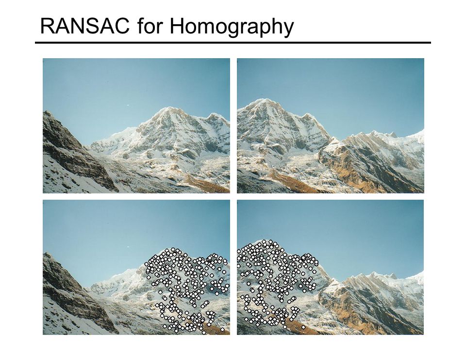
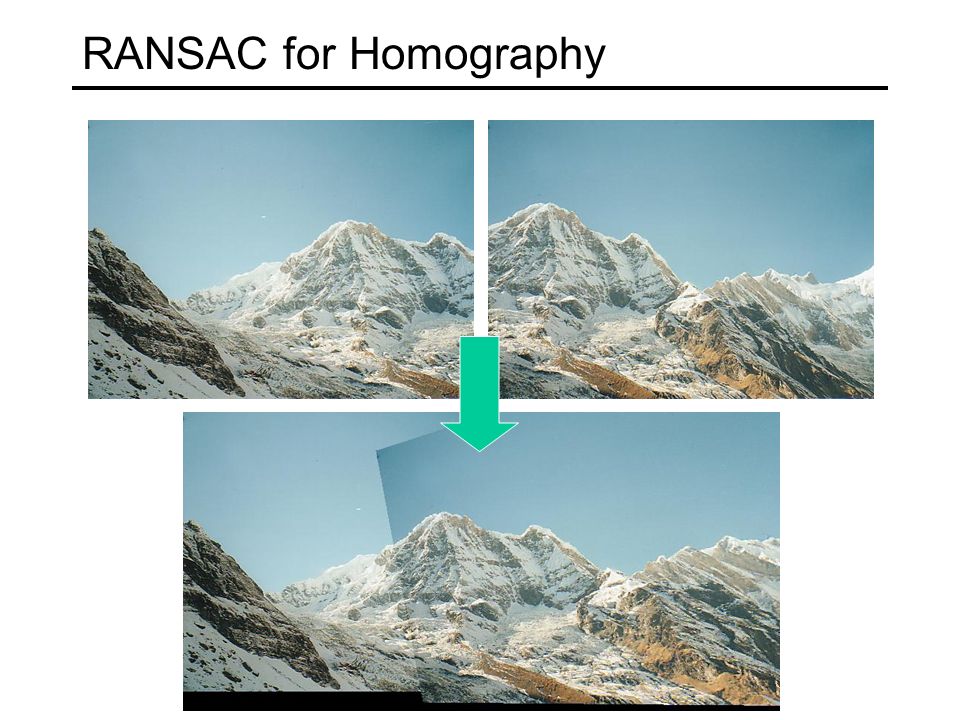
RANSAC for estimating homography RANSAC loop: 1.Select four feature pairs (at random) 2.Compute homography H (exact) 3.Compute inliers where SSD(p i ’, H p i) < ε 4.Keep largest set of inliers 5.Re-compute least-squares H estimate on all of the inliers
 2.Compute homography H (exact) 3.Compute inliers where SSD(p i ’, H p i) < ε 4.Keep largest set of inliers 5.Re-compute least-squares H estimate on all of the inliers")
56
RANSAC

57
Example: Recognising Panoramas M. Brown and D. Lowe, University of British Columbia

58
Why “Recognising Panoramas”?

59
1D Rotations ( ) Ordering matching images
 Ordering matching images")
60
Why “Recognising Panoramas”? 1D Rotations ( ) Ordering matching images
 Ordering matching images")
61
Why “Recognising Panoramas”? 1D Rotations ( ) Ordering matching images
 Ordering matching images")
62
Why “Recognising Panoramas”? 2D Rotations (, ) –Ordering matching images 1D Rotations ( ) Ordering matching images
 –Ordering matching images 1D Rotations ( ) Ordering matching images.")
63
Why “Recognising Panoramas”? 1D Rotations ( ) Ordering matching images 2D Rotations (, ) –Ordering matching images
 Ordering matching images 2D Rotations (, ) –Ordering matching images.")
64
Why “Recognising Panoramas”? 1D Rotations ( ) Ordering matching images 2D Rotations (, ) –Ordering matching images
 Ordering matching images 2D Rotations (, ) –Ordering matching images.")
65
Why “Recognising Panoramas”?

66
Overview Feature Matching Image Matching Bundle Adjustment Multi-band Blending Results Conclusions

67
RANSAC for Homography

70
Probabilistic model for verification

71
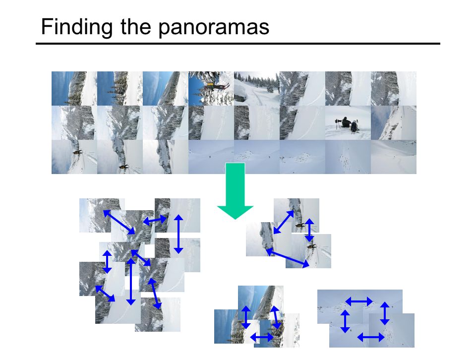
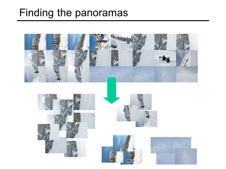
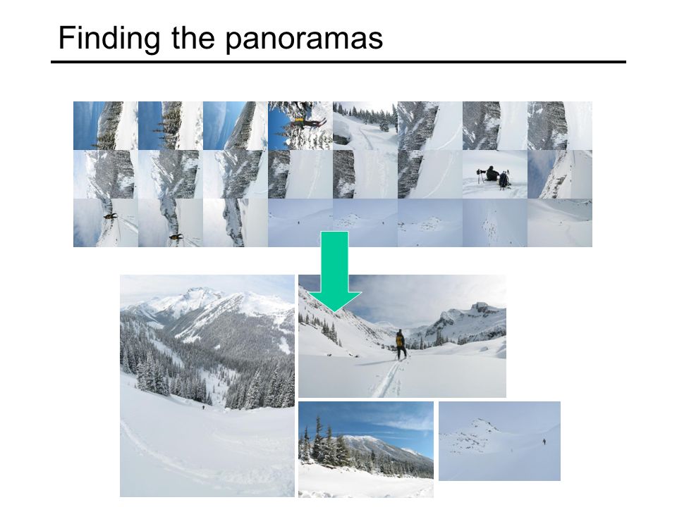
Finding the panoramas

75
Parameterise each camera by rotation and focal length This gives pairwise homographies Homography for Rotation

76
Bundle Adjustment New images initialised with rotation, focal length of best matching image

77
Bundle Adjustment New images initialised with rotation, focal length of best matching image

78
Multi-band Blending Burt & Adelson 1983 Blend frequency bands over range

79
Results

Similar presentations


 most slides from Steve Seitz,>")
>")

 Detector and Descriptor>")


 15-463: Computational Photography Alexei Efros, CMU, Fall 2006 with a lot of slides stolen from Steve Seitz and Rick.>")


 interest points, descriptors, Harris corners, correlation matching –Interest points.>")