1. Chapter No. 18 Radiation Detection and Measurements, Glenn T. Knoll, Third edition (2000), John Willey. Multichannel Pulse Analysis

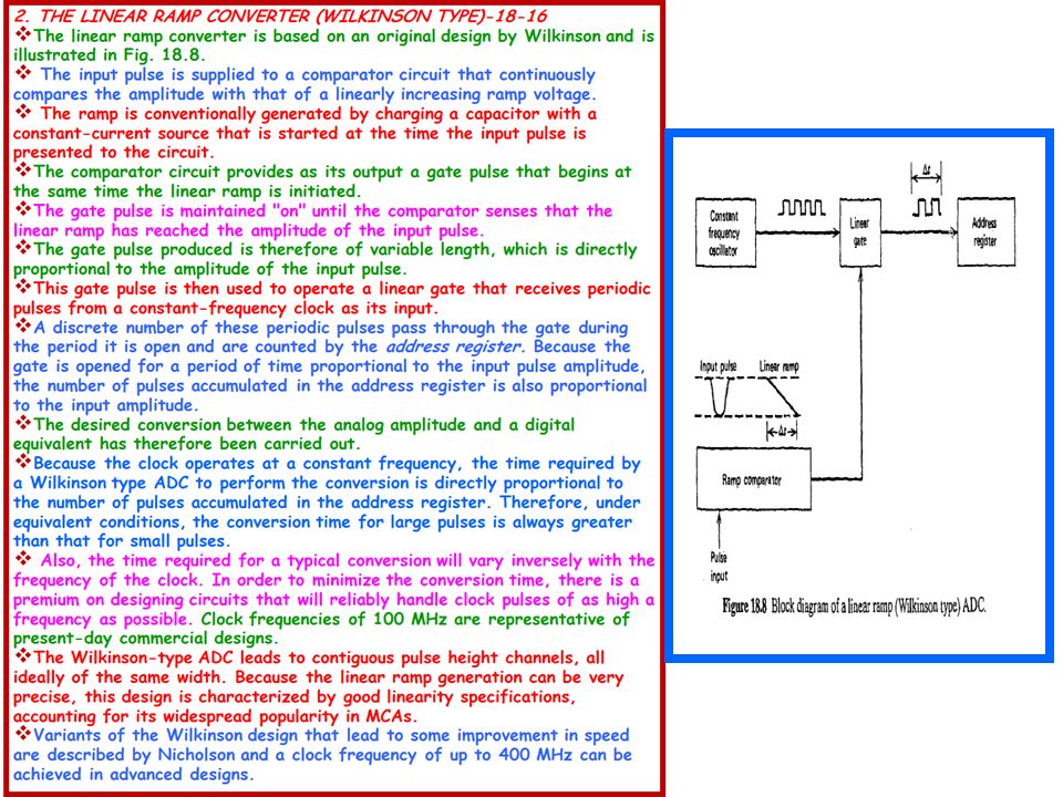
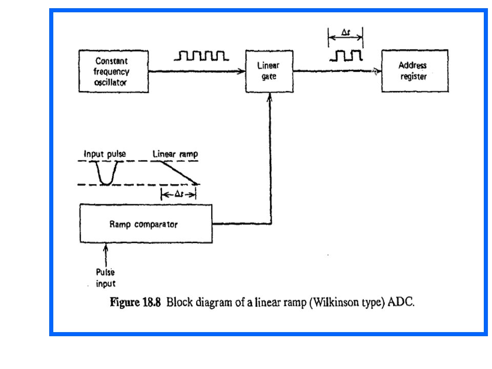
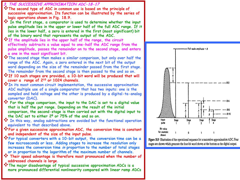
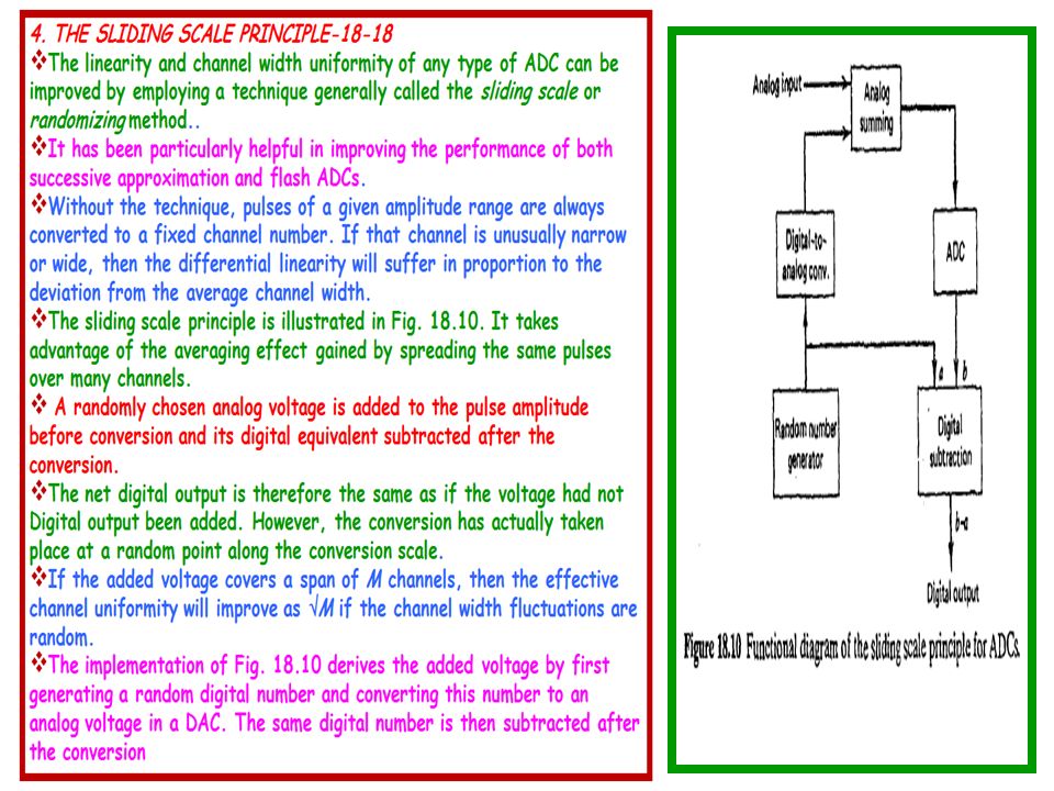
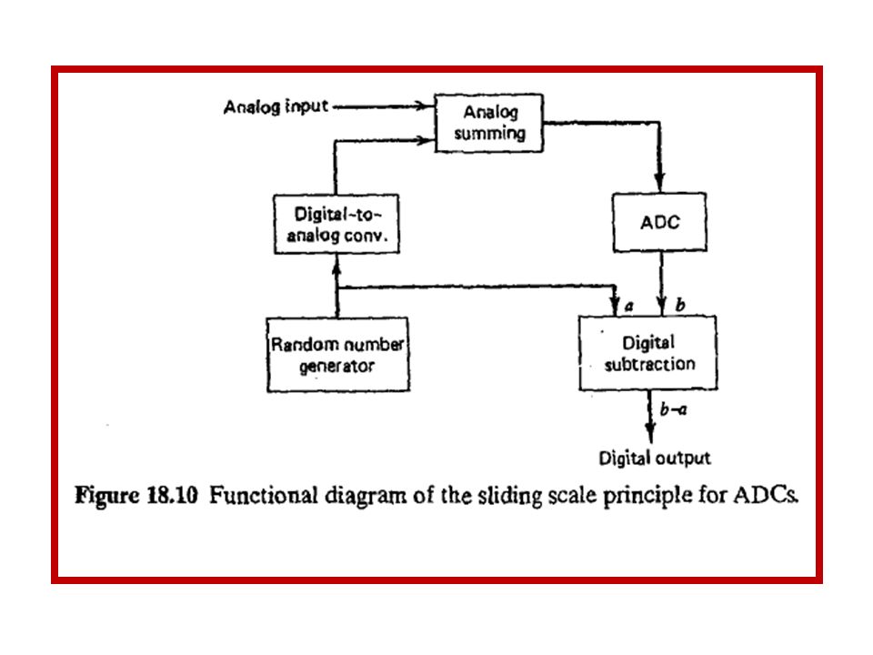
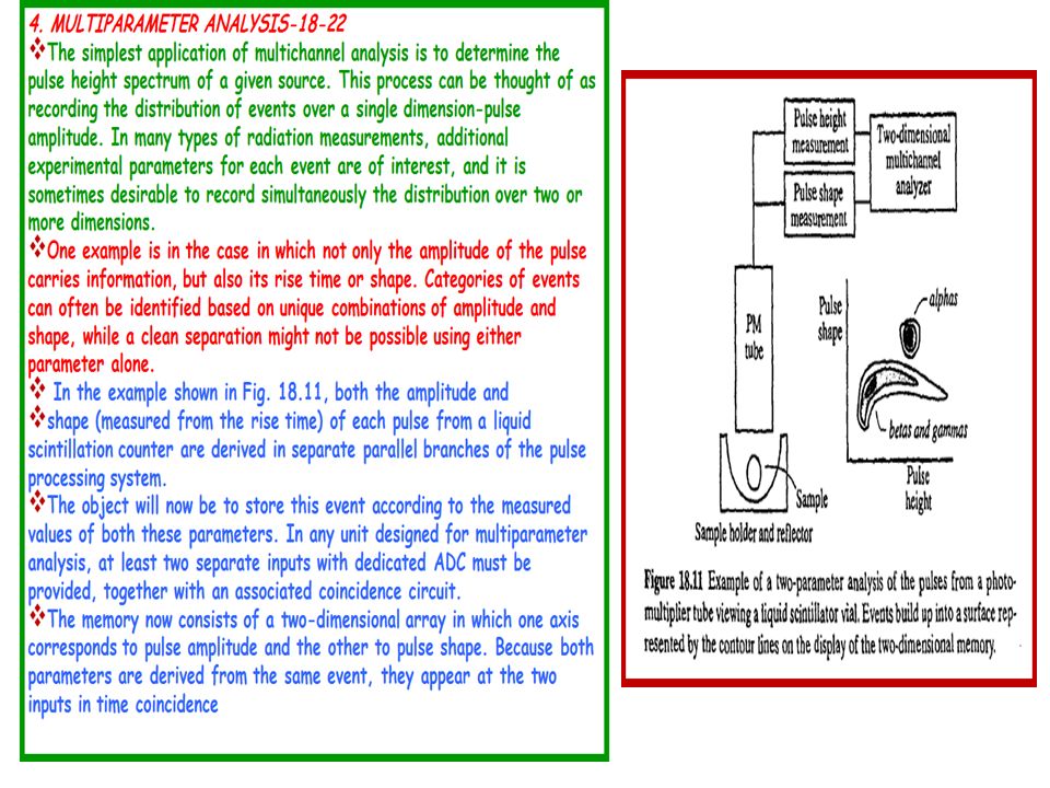
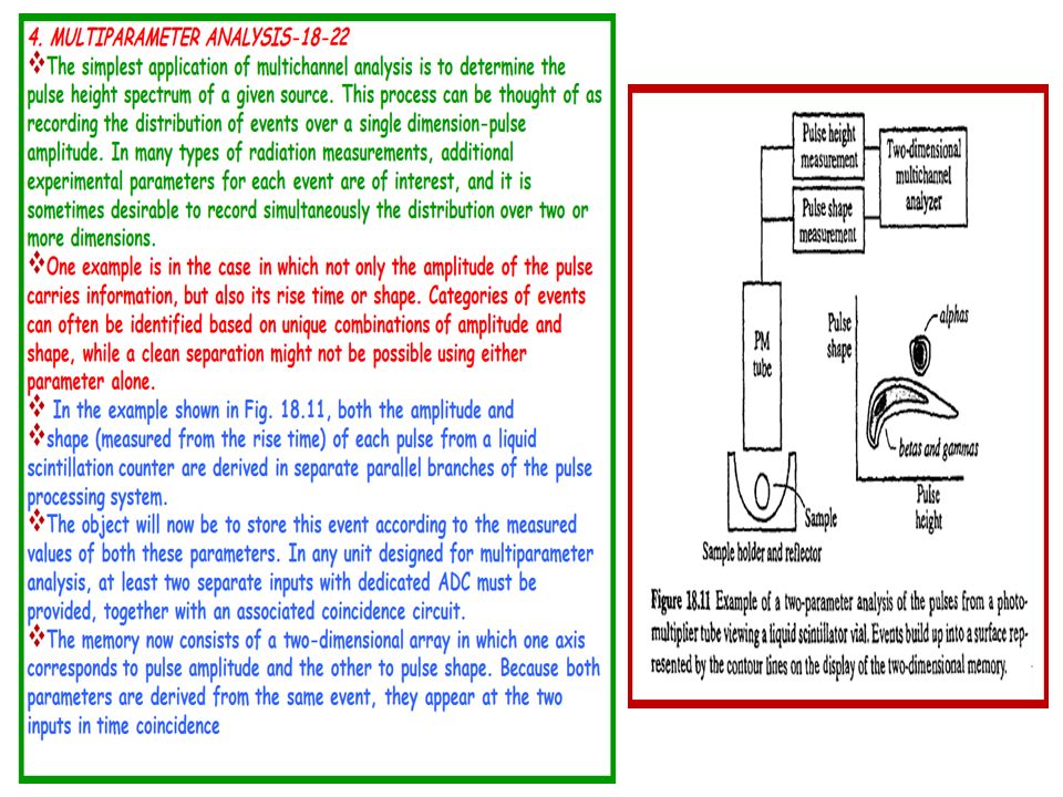
2. 2 Ch 18 GK I SINGLE·CHANNEL METHODS II GENERAL MULTICHANNEL CHARACTERISTICS  Number of Channels required  Calibration and linearity III THE MULTICHANNEL ANALYZER Basic components and functions  Analogue to digital converter  Linear Ramp Converter (Wilkinson type)  The Successive Approximation ADC  Sliding scale Principle  The Memory  Ancillory Functions  Multiscaling  Multiparameter Analysis  MCA dead time IV SPECTRUM STABILIZATION AND RELOCATION V SPECTRUM ANALYSIS

16.  18-13: If an MCA is operated at relatively high fractional dead time (say, greater than 30 or 40%), distortions in the spectrum can arise because of the greater probability of input pulses that arrive at the input gate just at the time it is either opening or closing.  It is therefore often advisable to reduce the counting rate presented to the input gate as much as possible by excluding noise and insignificant small- amplitude events with the LLD, and if significant numbers of large-amplitude background events are present, excluding them with an appropriate ULD setting.  The contents of the memory after a measurement can be displayed or recorded in a number of ways. Virtually all MCAs provide a CRT display of the content of each channel as the Y displacement versus the channel number as the X displacement. This display is therefore a graphical representation of the pulse height spectrum discussed earlier.  The display can be either on a linear vertical scale or, more commonly, as a logarithmic scale to show detail over a wider range of channel content. Standard recording devices for digital data, including printers and storage media, are commonly available to store permanently the memory content and to provide hard copy output.  Because of the similarity of many of the MCA components just described to those of the standard personal computer (PC), there is a widespread availability of plug-in cards that will convert a PC into an MCA.  The card must provide the components that are unique to the MCA (such as the ADC), but the normal PC memory, display, and I/O hardware can be used directly. Control of the MCA functions is then provided in the form of software that is loaded into the PC memory.

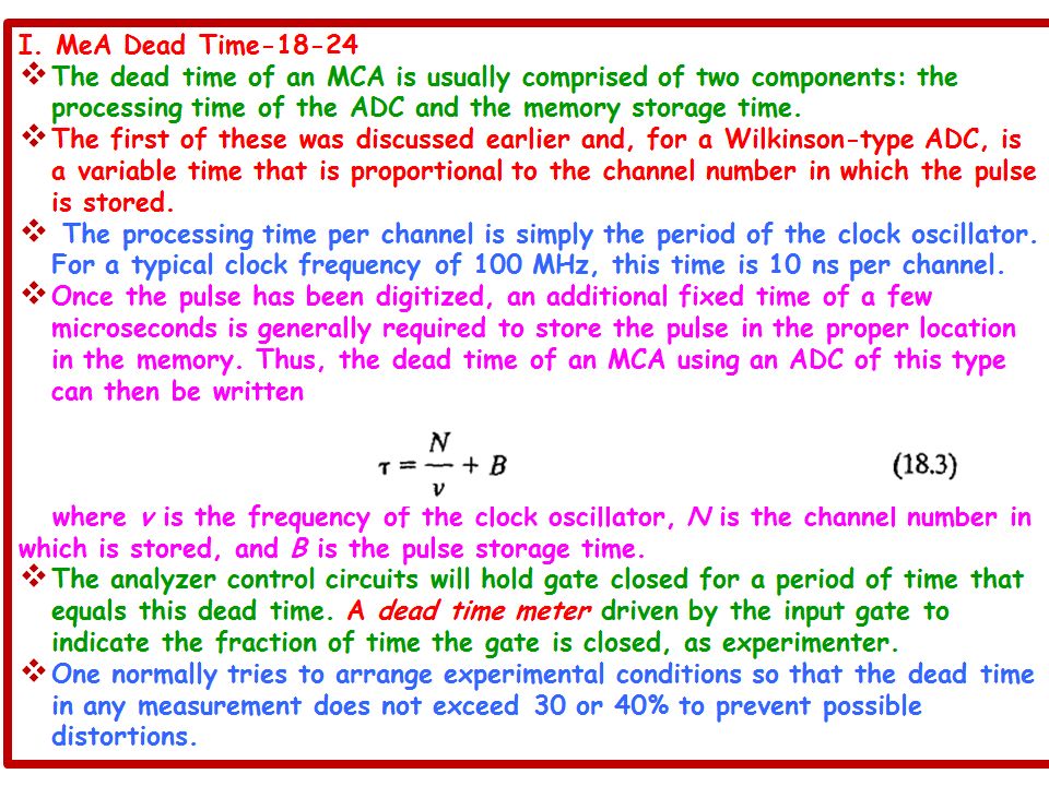
32. I. MeA Dead Time-18-24  The dead time of an MCA is usually comprised of two components: the processing time of the ADC and the memory storage time.  The first of these was discussed earlier and, for a Wilkinson-type ADC, is a variable time that is proportional to the channel number in which the pulse is stored.  The processing time per channel is simply the period of the clock oscillator. For a typical clock frequency of 100 MHz, this time is 10 ns per channel.  Once the pulse has been digitized, an additional fixed time of a few microseconds is generally required to store the pulse in the proper location in the memory. Thus, the dead time of an MCA using an ADC of this type can then be written where v is the frequency of the clock oscillator, N is the channel number in which is stored, and B is the pulse storage time.  The analyzer control circuits will hold gate closed for a period of time that equals this dead time. A dead time meter driven by the input gate to indicate the fraction of time the gate is closed, as experimenter.  One normally tries to arrange experimental conditions so that the dead time in any measurement does not exceed 30 or 40% to prevent possible distortions.

34.  18-25: The automatic live time operation of an MCA described earlier is usually quite satisfactory for making routine dead time corrections.  Circumstances can arise, however which the built-in live time correction is not accurate. When the fractional dead time high, errors can enter because the clock pulses are not generally of the same shape duration as signal pulses.  One remedy is to use the pulser technique to produce an artificial peak in the recorded spectrum. If introduced at the preamp the artificial pulses undergo the same amplification and shaping stages as the signal pulse  The fraction that are recorded then can account for both the losses due to pileup and analyzer dead time.  To avoid potential problems, the pulse repetition rate must not be too high, and the use of a random rather than periodic pulser is preferred.  Under these conditions, the pulser method can successfully handle virtually any conceivable case in which the shape of the spectrum does not change during the course of the measurement.  Additional complications arise if spectrum shape changes occur during the measurement, which lead to distortions and improper dead time corrections with the pulser method.