1. Computational Divided Differencing Thomas Reps University of Wisconsin Joint work with Louis B. Rall

2. Program Transformation Transform F  F # For all x, F(x) and F # (x) perform related computations Sometimes F # needs x to be preprocessed –F # (h(x))

3. int Sum() { int sum = 0; int i = 1; while (i < 11) { sum = sum + i; i = i + 1; } printf(“%d\n”,sum); printf(“%d\n”,i); } Example 1: Program Slicing Backward slice with respect to “ printf(“%d\n”,i) ”

4. int Sum() { int sum = 0; int i = 1; while (i < 11) { sum = sum + i; i = i + 1; } printf(“%d\n”,sum); printf(“%d\n”,i); } Example 1: Program Slicing Backward slice with respect to “ printf(“%d\n”,i) ”

5. int Sum_Select_i() { int i = 1; while (i < 11) { i = i + 1; } printf(“%d\n”,i); } Example 1: Program Slicing Backward slice with respect to “ printf(“%d\n”,i) ”

6. int Sum() { int sum = 0; int i = 1; while (i < 11) { sum = sum + i; i = i + 1; } printf(“%d\n”,sum); printf(“%d\n”,i); } Example 1: Program Slicing Backward slice with respect to “ printf(“%d\n”,sum) ”

7. int Sum() { int sum = 0; int i = 1; while (i < 11) { sum = sum + i; i = i + 1; } printf(“%d\n”,sum); printf(“%d\n”,i); } Example 1: Program Slicing Backward slice with respect to “ printf(“%d\n”,sum) ”

8. int Sum_Select_sum() { int sum = 0; int i = 1; while (i < 11) { sum = sum + i; i = i + 1; } printf(“%d\n”,sum); } Example 1: Program Slicing Backward slice with respect to “ printf(“%d\n”,sum) ”

9. Example 1: Program Slicing Given –F: program –  : projection function Create F , such that – F  (x) = (   F) (x) Sum Select[i] (x) = (Select[i]  Sum)(x) Sum Select[sum] (x) = (Select[sum]  Sum)(x)

10. Forward Slice int Sum() { int sum = 0; int i = 1; while (i < 11) { sum = sum + i; i = i + 1; } printf(“%d\n”,sum); printf(“%d\n”,i); } Forward slice with respect to “ sum = 0 ”

11. Forward Slice int Sum() { int sum = 0; int i = 1; while (i < 11) { sum = sum + i; i = i + 1; } printf(“%d\n”,sum); printf(“%d\n”,i); }

12. Who Cares About Slices? Understanding programs Restructuring Programs Program Specialization and Reuse Program Differencing Testing (and Retesting) Year 2000 Problem Automatic Differentiation

13. What Are Slices Useful For? Understanding Programs –What is affected by what? Restructuring Programs –Isolation of separate “computational threads” Program Specialization and Reuse –Slices = specialized programs –Only reuse needed slices Program Differencing –Compare slices to identify changes Testing –What new test cases would improve coverage? –What regression tests must be rerun after a change?

14. Example 2: Partial Evaluation Given – F: D 1  D 2  D 3 – s : D 1 Create F s : D 2  D 3, such that, –F s (d) = F(  s,d  ) F s (d) = F s (second(  s,d  )) = F(  s,d  )

15. Example 2: Partial Evaluation for(each pixel p){ Ray r = Ray(eye,p); Trace(object,r); } Trace(,r);  –

16. Example 2: Partial Evaluation for(each pixel p){ Ray r = Ray(eye,p); Trace(object,r); } Trace(,r);  –

17. Example 2: Partial Evaluation TraceObj = PEval(Trace,object); for(each pixel p){ Ray r = Ray(eye,p); TraceObj(r); }

18. Example 2: Partial Evaluation TraceObj = PEval(Trace,object); for(each pixel p){ Ray r = Ray(eye,p); TraceObj(r); }

19. Line-Character-Count Program void line_char_count(FILE *f) { int lines = 0; int chars; BOOL eof_flag = FALSE; int n; extern void scan_line (FILE *f, BOOL *bptr, int *iptr); scan_line(f, &eof_flag, &n); chars = n; while(eof_flag == FALSE){ lines = lines + 1; scan_line(f, &eof_flag, &n); chars = chars + n; } printf(“lines = %d\n”, lines); printf(“chars = %d\n”, chars); }

20. Character-Count Program void char_count(FILE *f) { int lines = 0; int chars; BOOL eof_flag = FALSE; int n; extern void scan_line (FILE *f, BOOL *bptr, int *iptr); scan_line(f, &eof_flag, &n); chars = n; while(eof_flag == FALSE){ lines = lines + 1; scan_line(f, &eof_flag, &n); chars = chars + n; } printf(“lines = %d\n”, lines); printf(“chars = %d\n”, chars); }

21. Line-Character-Count Program void line_char_count(FILE *f) { int lines = 0; int chars; BOOL eof_flag = FALSE; int n; extern void scan_line (FILE *f, BOOL *bptr, int *iptr); scan_line(f, &eof_flag, &n); chars = n; while(eof_flag == FALSE){ lines = lines + 1; scan_line(f, &eof_flag, &n); chars = chars + n; } printf(“lines = %d\n”, lines); printf(“chars = %d\n”, chars); }

22. Line-Count Program void line_count(FILE *f) { int lines = 0; int chars; BOOL eof_flag = FALSE; int n; extern void scan_line2 (FILE *f, BOOL *bptr, int *iptr); scan_line2(f, &eof_flag, &n); chars = n; while(eof_flag == FALSE){ lines = lines + 1; scan_line2(f, &eof_flag, &n); chars = chars + n; } printf(“lines = %d\n”, lines); printf(“chars = %d\n”, chars); }

23. Specialization Via Slicing wc -lc wc -c wc -l void line_char_count(FILE *f); Not partial evaluation!

24. Ex. 3: Computational Differentiation [“Automatic Differentiation”] Transform F  F’ F(x0)F(x0)  F(x0)F(x0) d dx F’(x 0 ) Comp. Diff.  F’(x0)F’(x0)

25. Computational Differentiation

26. float F(float x) { int i; float ans = 1.0; for(i = 1; i <= n; i++) { ans = ans * f[i](x); } return ans; } float delta =...; /* small constant */ float F’(float x) { return (F(x+delta) - F(x)) / delta; }

27. Computational Differentiation float F (float x) { int i; float ans = 1.0; for(i = 1; i <= n; i++) { ans = ans * f[i](x); } return ans ; }

28. Computational Differentiation float F’(float x) { int i; float ans’ = 0.0; float ans = 1.0; for(i = 1; i <= n; i++) { ans’ = ans * f’[i](x) + ans’ * f[i](x); ans = ans * f[i](x); } return ans’; }

29. Computational Differentiation ans’ = ans * f’[i](x) + ans’ * f[i](x); ans = ans * f[i](x); 0 0 1 1 f 1 ’(x) f 1 (x) 2 f 1 *f 2 ’ + f 1 ’*f 2 f 1 *f 2 3 f 1 *f 2 *f 3 ’ + f 1 *f 2 ’*f 3 + f 1 ’*f 2 *f 3 f 1 *f 2 *f 3 …...... Iter. ans’ ans

30. Differentiation Arithmetic class FloatD { public: float val'; float val; FloatD(float); }; FloatD operator+(FloatD a, FloatD b) { FloatD ans; ans.val' = a.val' + b.val'; ans.val = a.val + b.val; return ans; }

31. Differentiation Arithmetic class FloatD { public: float val'; float val; FloatD(float); }; FloatD operator*(FloatD a, FloatD b) { FloatD ans; ans.val' = a.val * b.val' + a.val' * b.val; ans.val = a.val * b.val; return ans; }

32. Differentiation Arithmetic float F(float x) { int i; float ans = 1.0; for(i = 1; i <= n; i++) { ans = ans * f[i](x); } return ans; }

33. Differentiation Arithmetic FloatD F(FloatD x) { int i; FloatD ans = 1.0; for(i = 1; i <= n; i++) { ans = ans * f[i](x); } return ans; }

34. Differentiation Arithmetic FloatD F(FloatD x) { int i; FloatD ans = 1.0; // ans.val’ = 0.0 // ans.val = 1.0 for(i = 1; i <= n; i++) { ans = ans * f[i](x); } return ans; }

35. Differentiation Arithmetic FloatD F(FloatD x) { int i; FloatD ans = 1.0; for(i = 1; i <= n; i++) { ans = ans * f[i](x); } return ans; } Similarly transformed version of f[i]

36. Differentiation Arithmetic FloatD F(FloatD x) { int i; FloatD ans = 1.0; for(i = 1; i <= n; i++) { ans = ans * f[i](x); } return ans; } Overloaded operator*

37. Differentiation Arithmetic FloatD F(FloatD x) { int i; FloatD ans = 1.0; for(i = 1; i <= n; i++) { ans = ans * f[i](x); } return ans; } Overloaded operator=

38. Laws for F’ c’ = 0 x’ = 1 (c + F)’(x) = F’(x) (c * F)’(x) = c * F’(x) (F + G)’(x) = F’(x) + G’(x) (F * G)’(x) = F’(x) * G(x) + F(x) * G’(x)

39. Differentiation Arithmetic F vF(v) Differentiating version of F vF(v) wF ’ (v)*w Computational Differentiation

40. Chain Rule G v G(v) F F(G(v)) Computational Differentiation v 1.0 Differentiating version of G G(v) G ’ (v) Computational Differentiation F(G(v)) F’(G(v))*G ’ (v) Differentiating version of F

41. Computational Differentiation x1x1 xixi xmxm y1y1 y j+1 ynyn Program Chopping x2x2 x i+1 y2y2 yjyj x2x2 y2y2 yjyj y = F(x)

42. The If Problem float F(float x) { float ans; if (x == 1.0) { ans = 1.0; } else { ans = x*x; } return ans; }

43. The If Problem float F’(float x) { float ans'; float ans; if (x == 1.0) { ans' = 0.0; ans = 1.0; } else { ans' = x+x; ans = x*x; } return ans'; } F’(1.0) = 0.0 versus F ’ (1.0) = 2.0

44. Outline Programs as data objects –Partial evaluation –Slicing –Computational differentiation (CD) Computational divided differencing CDD generalizes CD Higher-order CDD Multi-variate CDD

45. Accurate Computation of Divided Differences

46. Divided Differences = Slopes x1x1 F(x1)F(x1) x0x0 F(x0)F(x0) F

47. Who Cares About Divided Differences? Interpolation/extrapolation Numerical integration Solving differential equations Scientific and graphics programs: Predict and render modeled situations

48. Computing Divided Differences float Square(float x) { return x * x; } float Square_1DD_naive(float x0,float x1) { return (Square(x0) - Square(x1))/(x0 - x1); } round-off error! division by a small quantity No Way!

49. Consider F(x) = x 2, when x 0  x 1 But … x02 – x12x0 – x1x02 – x12x0 – x1 = F [x 0, x 1 ] = F(x 0 ) – F(x 1 ) x 0 – x 1 = x 0 + x 1

50. Computing Divided Differences float Square(float x) { return x * x; } float Square_1DD_naive(float x0,float x1) { return (Square(x0) - Square(x1))/(x0 - x1); } float Square_1DD(float x0,float x1) { return x0 + x1; }

51. Example: Evaluation via Horner's rule class Poly { public: Poly(int N, float x[]); float Eval(float); private: int degree; float *coeff; // Array coeff[0..degree] }; P(x) = 2.1 * x 3 – 1.4 * x 2 –.6 * x + 1.1 Poly *P = new Poly(4,2.1,-1.4,-0.6,1.1); float val = P->Eval(3.005); P(x) = ((((0.0 * x + 2.1) * x – 1.4) * x –.6) * x + 1.1)

52. Example: Evaluation via Horner's rule float Poly::Eval(float x) { int i; float ans = 0.0; for (i = degree; i >= 0; i--) { ans = ans * x + coeff[i]; } return ans; } P(x) = ((((0.0 * x + 2.1) * x – 1.4) * x –.6) * x + 1.1)

53. Example: Evaluation via Horner's rule float Poly::Eval_1DD(float x0,float x1) { int i; float ans_1DD = 0.0; float ans = 0.0; for (i = degree; i >= 0; i--) { ans_1DD = ans_1DD * x1 + ans; ans = ans * x0 + coeff[i]; } return ans_1DD; } P(x) = ((((0.0 * x + 2.1) * x – 1.4) * x –.6) * x + 1.1)

54. Laws for F[x 0,x 1 ] c’ = 0 x’ = 1 (c+F)’(x) = F’(x) (c*F)’(x) = c*F’(x) (F+G)’(x) = F’(x)+G’(x) (F*G)’(x) = F’(x)*G(x) + F(x)*G’(x) c[x 0,x 1 ] = 0 x[x 0,x 1 ] = 1 (c+F)[x 0,x 1 ] = F [x 0,x 1 ] (c*F)[x 0,x 1 ] = c*F[x 0,x 1 ] (F+G)[x 0,x 1 ] = F[x 0,x 1 ]+G[x 0,x 1 ] (F*G) [x 0,x 1 ] = F [x 0,x 1 ]*G(x 1 ) + F(x 0 )*G[x 0,x 1 ]

55. Outline Programs as data objects –Partial evaluation –Slicing –Computational differentiation (CD) Computational divided differencing CDD generalizes CD Higher-order CDD Multi-variate CDD

56. F(x0)F(x0)  F(x0)F(x0) F [x 0, x 1 ] F(x 0 ) - F(x 1 ) x 0 - x 1 d dx F’(x 0 ) Comp. Diff.  F’(x0)F’(x0) F(x 0 )-F(x 1 ) x 0 -x 1 Standard Div. Diff. x1x0x1x0 ? x1x0x1x0

57. F(x0)F(x0)  F(x0)F(x0) F [x 0, x 1 ] F(x 0 ) - F(x 1 ) x 0 - x 1 d dx F’(x 0 ) Comp. Diff.  F’(x0)F’(x0) F[x0,x1]F[x0,x1] Comp. Div. Diff. x1x0x1x0 x1x0x1x0

58. First Divided Difference if x 0  x 1 F[x 0, x 0 ] = d dz F(z)F(z) z = x 0

59. Laws for F[x 0,x 1 ] c’ = 0 x’ = 1 (c+F)’(x) = F’(x) (c*F)’(x) = c*F’(x) (F+G)’(x) = F’(x)+G’(x) (F*G)’(x) = F’(x)*G(x) + F(x)*G’(x) c[x 0,x 1 ] = 0 x[x 0,x 1 ] = 1 (c+F)[x 0,x 1 ] = F [x 0,x 1 ] (c*F)[x 0,x 1 ] = c*F[x 0,x 1 ] (F+G)[x 0,x 1 ] = F[x 0,x 1 ]+G[x 0,x 1 ] (F*G) [x 0,x 1 ] = F [x 0,x 1 ]*G(x 1 ) + F(x 0 )*G[x 0,x 1 ]

60. Laws for F[x 0,x 0 ] c’ = 0 x’ = 1 (c+F)’(x) = F’(x) (c*F)’(x) = c*F’(x) (F+G)’(x) = F’(x)+G’(x) (F*G)’(x) = F’(x)*G(x) + F(x)*G’(x) c[x 0,x 0 ] = 0 x[x 0,x 0 ] = 1 (c+F)[x 0,x 0 ] = F [x 0,x 0 ] (c*F)[x 0,x 0 ] = c*F[x 0,x 0 ] (F+G)[x 0,x 0 ] = F[x 0,x 0 ]+G[x 0,x 0 ] (F*G) [x 0,x 0 ] = F [x 0,x 0 ]*G(x 0 ) + F(x 0 )*G[x 0,x 0 ]

61. Example: Evaluation via Horner's rule float Poly::Eval(float x) { int i; float ans = 0.0; for (i = degree; i >= 0; i--) { ans = ans * x + coeff[i]; } return ans; }

62. Example: Evaluation via Horner's rule float Poly::Eval_1DD(float x0,float x1) { int i; float ans_1DD = 0.0; float ans = 0.0; for (i = degree; i >= 0; i--) { ans_1DD = ans_1DD * x1 + ans; ans = ans * x0 + coeff[i]; } return ans_1DD; }

63. Example: Evaluation via Horner's rule float Poly::Eval_1DD(float x0,float x1) { int i; float ans_1DD = 0.0; float ans = 0.0; for (i = degree; i >= 0; i--) { ans_1DD = ans_1DD * v + ans; ans = ans * v + coeff[i]; } return ans_1DD; } v v

64. Example: Evaluation via Horner's rule float Poly::Eval'(float x) { int i; float ans' = 0.0; float ans = 0.0; for (i = degree; i >= 0; i--) { ans' = ans' * x + ans; ans = ans * x + coeff[i]; } return ans'; }

65. Example: Evaluation via Horner's rule float Poly::Eval'(float x) { int i; float ans' = 0.0; float ans = 0.0; for (i = degree; i >= 0; i--) { ans' = ans' * v + ans; ans = ans * v + coeff[i]; } return ans'; } Eval_1DD(v,v) = = Eval’(v) v

66. Outline Programs as data objects –Partial evaluation –Slicing –Computational differentiation (CD) Computational divided differencing CDD generalizes CD Higher-order CDD Multi-variate CDD

67. Accurate Computation of Divided Differences

68. F [x 0, x 1, x 2 ]: Slopes of Slopes x2x2 F(x2)F(x2) x1x1 F(x1)F(x1) F x0x0 F(x0)F(x0)

69. Divided-Difference Table F(x 0 ) F[x 0,x 1 ] F(x 1 ) F[x 0,x 1,x 2 ] F[x 1,x 2 ] F[x 0,x 1,x 2,x 3 ] F(x 2 ) F[x 1,x 2,x 3 ] F[x 2,x 3 ] F(x 3 )

70. F(x 0 )F[x 0,x 1 ]F[x 0,x 1,x 2 ] F[x 0,x 1,x 2,x 3 ] F(x 1 )F[x 1,x 2 ] F[x 1,x 2,x 3 ] F(x 2 ) F[x 2,x 3 ] F(x 3 ) 0 0 00 Divided-Difference Table F  [x 0, x 1, x 2, x 3 ]

71. Laws for F  [x 0,…,x n ] c  = c*I x  = A [x0,…,xn] (c+F)  (x) = F  (x) (c*F)  (x) = c*F  (x) (F+G)  (x) = F  (x)+G  (x) (F*G)  (x) = F  (x)*G  (x) c[x 0,x 1 ] = 0 x[x 0,x 1 ] = 1 (c+F)[x 0,x 1 ] = F’[x 0,x 1 ] (c*F)[x 0,x 1 ] = c*F[x 0,x 1 ] (F+G)[x 0,x 1 ] = F[x 0,x 1 ]+G[x 0,x 1 ] (F*G) [x 0,x 1 ] = F [x 0,x 1 ]*G(x 1 ) + F(x 0 )*G[x 0,x 1 ]

72. 2.1  = 2.1 * I 2.1 0.0 0.0 0.0 2.1 0.0 0.0 2.1 0.0 2.1

73. 3.0 1.0 0.0 0.0 4.0 1.0 0.0 5.0 1.0 7.0 x  = A [3,4,5,7] 2.1  = 2.1 * I 2.1 0.0 0.0 0.0 2.1 0.0 0.0 2.1 0.0 2.1

74. 2.1x 3 – 1.4x 2 –.6x + 1.1 43.467.323.8 2.09999 110.7114.9 32.2 225.6211.5 648.6 StandardStandard 43.467.323.8 2.1 110.7114.9 32.2 225.6211.5 648.6 CDDCDD x 0 : 3.0x 1 : 4.0x 2 : 5.0x 3 : 7.0

75. 2.1x 3 – 1.4x 2 –.6x + 1.1 43.447.717715.2886 754.685 43.447747.7483 19.0621 43.4955 47.8245 43.6389 StandardStandard x 0 : 3.0x 1 : 3.001x 2 : 3.002x 3 : 3.005 CDDCDD 43.447.717517.5063 2.1 43.447747.7525 17.5168 43.4955 47.8226 43.6389

76. 2.1x 3 – 1.4x 2 –.6x + 1.1 43.4 47.6945 3.62366 117520 43.4048 47.6942 62.379 43.4095 47.7202 43.4238 StandardStandard x 0 : 3.0 x 1 : 3.0001 x 2 : 3.0002 x 3 : 3.0005 CDDCDD 43.4 47.7017 17.5006 2.1 43.4048 47.7052 17.5017 43.4095 47.7122 43.4238

77. 2.1x 3 – 1.4x 2 –.6x + 1.1 43.4 NaN NaN NaN 43.4 NaN NaN 43.4 NaN 43.4 StandardStandard x 0 : 3.0 x 1 : 3.0 x 2 : 3.0 x 3 : 3.0 CDDCDD 43.4 47.7 17.5 2.1 43.4 47.7 17.5 43.4 47.7 43.4

78. Example: Evaluation via Horner's rule class Poly { public: Poly(int N, float x[]); float Eval(float); private: int degree; float *coeff; // Array coeff[0..degree] };

79. Example: Evaluation via Horner's rule class Poly { public: Poly(int N, float x[]); float Eval(float); FloatDD Eval(FloatDD); private: int degree; float *coeff; // Array coeff[0..degree] }; P(x) = 2.1 * x 3 – 1.4 * x 2 –.6 * x + 1.1 Poly *P = new Poly(4,2.1,-1.4,-0.6,1.1); FloatDD xs(4, 3.0, 4.0, 5.0, 7.0); FloatDD ddt = P->Eval(xs);

80. Example: Evaluation via Horner's rule float Poly::Eval(float x) { int i; float ans = 0.0; for (i = degree; i >= 0; i--) { ans = ans * x + coeff[i]; } return ans; }

81. Example: Evaluation via Horner's rule FloatDD Poly::Eval(FloatDD x) { int i; FloatDD ans = 0.0; for (i = degree; i >= 0; i--) { ans = ans * x + coeff[i]; } return ans; }

82. 2.1x 3 – 1.4x 2 –.6x + 1.1 3.0 1.0 0.0 0.0 4.0 1.0 0.0 5.0 1.0 7.0 x ans 0.0 0.0 0.0 0.0 0.0 0.0 0.0 0.0 0.0

83. 2.1x 3 – 1.4x 2 –.6x + 1.1 3.0 1.0 0.0 0.0 4.0 1.0 0.0 5.0 1.0 7.0 x ans 2.1 0.0 0.0 0.0 2.1 0.0 0.0 2.1 0.0 2.1

84. 2.1x 3 – 1.4x 2 –.6x + 1.1 3.0 1.0 0.0 0.0 4.0 1.0 0.0 5.0 1.0 7.0 x ans 4.9 2.1 0.0 0.0 7.0 2.1 0.0 9.1 2.1 13.3

85. 2.1x 3 – 1.4x 2 –.6x + 1.1 3.0 1.0 0.0 0.0 4.0 1.0 0.0 5.0 1.0 7.0 x ans 14.113.3 2.1 0.0 27.4 17.5 2.1 44.923.8 92.5

86. 2.1x 3 – 1.4x 2 –.6x + 1.1 3.0 1.0 0.0 0.0 4.0 1.0 0.0 5.0 1.0 7.0 x ans 43.467.323.8 2.1 110.7114.9 32.2 225.6211.5 648.6

87. Example: Plotting a Function x P(x) Evaluate CDD+Briggs Standard+Briggs 0.0000 1.10000 1.10000 1.10000 0.0001 1.09994 1.09994 1.09994 0.0002 1.09988 1.09988 1.09988 … … … … 0.9998 1.19942 1.19941 19844.3 0.9999 1.19971 1.19970 19850.3 1.0000 1.2 1.19999 19856.2 Time 7.64 5.62 5.49

88. Outline Programs as data objects –Partial evaluation –Slicing –Computational differentiation (CD) Computational divided differencing CDD generalizes CD Higher-order CDD Multi-variate CDD

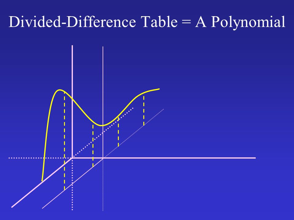
89. Divided-Difference Table = A Polynomial 2.1x 3 – 1.4x 2 –.6x + 1.1 43.467.323.8 2.1 110.7114.9 32.2 225.6211.5 648.6 CDDCDD x 0 : 3.0x 1 : 4.0x 2 : 5.0x 3 : 7.0

90. Newton Interpolating Polynomial … + (  (x – x j ) ) F[x 0,…,x m ] + … j=0 m–1m–1 … + d m dz m F(z)F(z) z = x 0 + … (x–x0)mm!(x–x0)mm!

91. CDDCDD 43.4 47.7 17.5 2.1 43.4 47.7 17.5 43.4 47.7 43.4 Divided-Difference Table = A Polynomial x 0 : 3.0 x 1 : 3.0 x 2 : 3.0 x 3 : 3.0 2.1x 3 – 1.4x 2 –.6x + 1.1

92. Taylor Series … + (x–x 0 ) m F[x 0,…,x 0 ] + … … + d m dz m F(z)F(z) z = x 0 + … (x–x0)mm!(x–x0)mm! m+1 x 0 ’s

93. Divided-Difference Table = A Polynomial = 

95. = 

98. Linear Interpolation

102. First Divided Difference = Slope x1x1 F(x1)F(x1) x0x0 F(x0)F(x0) F

103. Divided-Difference Table = A Polynomial  = 1  = 0 x1x1 x0x0

104. First Divided Difference = Slope x0x0 x1x1 –  1  0 x0 – x1x0 – x1

105. x0x0 x1x1 –  1  0 x0 – x1x0 – x1

106. Divided-Difference Table = A Surface x0x0 x1x1 -  1  0 x 0 - x 1  1  0 0

107. Avoid the Subtractions! -  1  0 x 0 - x 1  1  0 0 Use a divided-difference arithmetic: Divided-difference tables of divided-difference tables       *    =

108. Quadratic Interpolation

109. Divided-Difference Table = A Surface  1  0 0  2 0 0 -  0 x 0 - x 1  1 -  1 x 1 - x 2  2 -  0 x 0 - x 1  1 x 0 – x 2 – -  1 x 1 - x 2  2

110. Example: Evaluation via Horner's rule class BivariatePoly { public: float Eval(float,float); private: int degree1,degree2; // Array coeff[0..degree1][0..degree2] float **coeff; }; float val = P->Eval(x,y);

111. Example: Evaluation via Horner's rule float BivariatePoly::Eval(float x,float y) { float ans = 0.0; for (int i = degree1; i >= 0; i--) { float temp = 0.0; for (int j = degree2; j >= 0; j--) { temp = temp * y + coeff[i][j]; } ans = ans * x + temp; } return ans; }

112. Example: Evaluation via Horner's rule DDA BivariatePoly::Eval(DDA x, DDA y) { DDA ans = 0.0; for (int i = degree1; i >= 0; i--) { DDA temp = 0.0; for (int j = degree2; j >= 0; j--) { temp = temp * y + coeff[i][j]; } ans = ans * x + temp; } return ans; } DDA x(VAR, 1, x 0, x 1, x 2, x 3 ); DDA y(VAR, 2, y 0, y 1, y 2 ); DDA surface = P->Eval(x,y);

113. F(x 0 )F[x 0,x 1 ]F[x 0,x 1,x 2 ] F[x 0,x 1,x 2,x 3 ] F(x 1 )F[x 1,x 2 ] F[x 1,x 2,x 3 ] F(x 2 ) F[x 2,x 3 ] F(x 3 ) 0 0 00 Relationships Between CDD and CD F  [x 0, x 1, x 2, x 3 ]

114. F(x 0 )F[x 0,x 0 ]F[x 0,x 0,x 0 ] F[x 0,x 0,x 0,x 0 ] F(x 0 )F[x 0,x 0 ] F[x 0,x 0,x 0 ] F(x 0 ) F[x 0,x 0 ] F(x 0 ) 0 0 00 Relationships Between CDD and CD F  [x 0, x 0, x 0, x 0 ]

115. F(x 0 )F[x 0,x 0 ]F[x 0,x 0,x 0 ] F[x 0,x 0,x 0,x 0 ] F(x 0 )F[x 0,x 0 ] F[x 0,x 0,x 0 ] F(x 0 ) F[x 0,x 0 ] F(x 0 ) 0 0 00 Relationships Between CDD and CD Computational Differentiation

116. F(x 0 )F[x 0,x 0 ]F[x 0,x 0,x 0 ] F[x 0,x 0,x 0,x 0 ] F(x 0 )F[x 0,x 0 ] F[x 0,x 0,x 0 ] F(x 0 ) F[x 0,x 0 ] F(x 0 ) 0 0 00 Relationships Between CDD and CD Differentiation Arithmetic

117. F(x 0 )F[x 0,x 0 ]F[x 0,x 0,x 0 ] F[x 0,x 0,x 0,x 0 ] F(x 0 )F[x 0,x 0 ] F[x 0,x 0,x 0 ] F(x 0 ) F[x 0,x 0 ] F(x 0 ) 0 0 00 Relationships Between CDD and CD Taylor-Coefficient Arithmetic

118. Related Work Computational differentiation –Wengert, Rall, Iri, Griewank, Bischof, Carle, … Accurate divided differencing –Matrix operations: Opitz 64 (McCurdy 80, Reps 98) –Library functions: McCurdy 80, Kahan & Fateman 85, Rall & Reps 00 Controlling round-off error –Kulisch’s group at Karlsruhe Operator overloading –partial evaluation, safe pointers, expression templates