Download presentation
Presentation is loading. Please wait.

1
Quicksort Quicksort is a well-known sorting algorithm that, in the worst case, it makes Θ(n 2 ) comparisons. Typically, quicksort is significantly faster in practice than other Θ(nlogn) algorithms, because its inner loop can be efficiently implemented on most architectures, and in most real-world data it is possible to make design choices which minimize the possibility of requiring quadratic time. Quicksort is a comparison sort and, in efficient implementations, is not a stable sort.
 algorithms, because its inner loop can be efficiently implemented on most architectures, and in most real-world data it is possible to make design choices which minimize the possibility of requiring quadratic time. Quicksort is a comparison sort and, in efficient implementations, is not a stable sort..")
2
History The quicksort algorithm was developed by C. A. R. Hoare in 1960 while working for the small British scientific computer manufacturer Elliott Brothers.

3
Algorithm Quicksort sorts by employing a divide and conquer strategy to divide a list into two sub-lists. The steps are: Pick an element, called a pivot, from the list. Reorder the list so that all elements which are less than the pivot come before the pivot and so that all elements greater than the pivot come after it (equal values can go either way). After this partitioning, the pivot is in its final position. This is called the partition operation. Recursively sort the sub-list of lesser elements and the sub-list of greater elements. The base case of the recursion are lists of size zero or one, which are always sorted.
. After this partitioning, the pivot is in its final position. This is called the partition operation. Recursively sort the sub-list of lesser elements and the sub-list of greater elements. The base case of the recursion are lists of size zero or one, which are always sorted..")
4
Pseudocode function quicksort(array, left, right) if right > left select a pivot index (e.g. pivotIndex := left) pivotNewIndex := partition(array, left, right, pivotIndex) quicksort(array, left, pivotNewIndex - 1) quicksort(array, pivotNewIndex + 1, right)
 pivotNewIndex := partition(array, left, right, pivotIndex) quicksort(array, left, pivotNewIndex - 1) quicksort(array, pivotNewIndex + 1, right).")
5
Pseudocode for Partition function partition(array, left, right, pivotIndex) pivotValue := array[pivotIndex] swap array[pivotIndex] and array[right] // Move pivot to end storeIndex := left for i from left to right // left ≤ i < right if array[i] ≤ pivotValue swap array[i] and array[storeIndex] storeIndex := storeIndex + 1 swap array[storeIndex] and array[right] // Move pivot to its final place return storeIndex
![Pseudocode for Partition function partition(array, left, right, pivotIndex) pivotValue := array[pivotIndex] swap array[pivotIndex] and array[right] // Move pivot to end storeIndex := left for i from left to right // left ≤ i < right if array[i] ≤ pivotValue swap array[i] and array[storeIndex] storeIndex := storeIndex + 1 swap array[storeIndex] and array[right] // Move pivot to its final place return storeIndex](http://images.slideplayer.com/32/9831220/slides/slide_5.jpg "Pseudocode for Partition function partition(array, left, right, pivotIndex) pivotValue := array[pivotIndex] swap array[pivotIndex] and array[right] // Move pivot to end storeIndex := left for i from left to right // left ≤ i < right if array[i] ≤ pivotValue swap array[i] and array[storeIndex] storeIndex := storeIndex + 1 swap array[storeIndex] and array[right] // Move pivot to its final place return storeIndex")
6
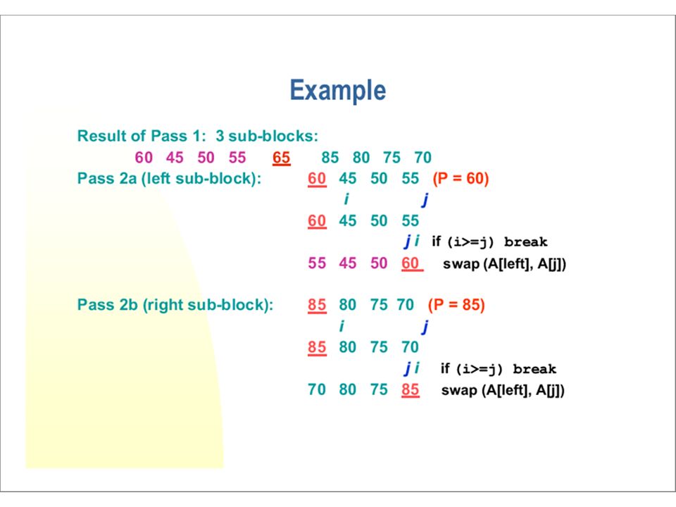
Basic Ideas (Divide-and-conquer algorithm) Pick an element, say P(the pivot) Re-arrange the elements into 3 sub-blocks, 1.those less than or equal to (≤) P(the left-block S1) 2.P(the only element in the middle-block) 3.those greater than or equal to (≥) P(the right-block S2) Repeat the process recursively for the left-and right-sub- blocks. Return {quicksort(S1), P, quicksort(S2)}.(That is the results of quicksort(S1), followed by P, followed by the results of quicksort(S2))
, P, quicksort(S2)}.(That is the results of quicksort(S1), followed by P, followed by the results of quicksort(S2)).")
7
Implementation Algorithm int partition (int A[ ], int left, int right); // sort A[left..right]void quicksort(int A[ ], int left, int right) { int q ; if (right > left ) { q = partition(A, left, right); // after ‘partition’ //A[left..q-1] ≤A[q] ≤A[q+1..right] quicksort(A, left, q-1); quicksort(A, q+1, right); }
![Implementation Algorithm int partition (int A[ ], int left, int right); // sort A[left..right]void quicksort(int A[ ], int left, int right) { int q ; if (right > left ) { q = partition(A, left, right); // after ‘partition’ //A[left..q-1] ≤A[q] ≤A[q+1..right] quicksort(A, left, q-1); quicksort(A, q+1, right); }](http://images.slideplayer.com/32/9831220/slides/slide_7.jpg "Implementation Algorithm int partition (int A[ ], int left, int right); // sort A[left..right]void quicksort(int A[ ], int left, int right) { int q ; if (right > left ) { q = partition(A, left, right); // after ‘partition’ //A[left..q-1] ≤A[q] ≤A[q+1..right] quicksort(A, left, q-1); quicksort(A, q+1, right); }")
8
// select A[left] be the pivot element) int partition(int A[], int left, int right); { P = A[left]; i = left; j = right + 1; for(;;)//infinite for-loop, break to exit { while(A[++i] = right) break; // Now, A[i] ≥P while(A[--j] > P) if (j <= left) break; // Now, A[j] ≤P if (i >= j ) break; // break the for-loop else swap(A[i], A[j]); } if (j == left) return j ; swap(A[left], A[j]); return j; }
![// select A[left] be the pivot element) int partition(int A[], int left, int right); { P = A[left]; i = left; j = right + 1; for(;;)//infinite for-loop, break to exit { while(A[++i] = right) break; // Now, A[i] ≥P while(A[--j] > P) if (j <= left) break; // Now, A[j] ≤P if (i >= j ) break; // break the for-loop else swap(A[i], A[j]); } if (j == left) return j ; swap(A[left], A[j]); return j; }](http://images.slideplayer.com/32/9831220/slides/slide_8.jpg "// select A[left] be the pivot element) int partition(int A[], int left, int right); { P = A[left]; i = left; j = right + 1; for(;;)//infinite for-loop, break to exit { while(A[++i] = right) break; // Now, A[i] ≥P while(A[--j] > P) if (j <= left) break; // Now, A[j] ≤P if (i >= j ) break; // break the for-loop else swap(A[i], A[j]); } if (j == left) return j ; swap(A[left], A[j]); return j; }")
13
So the trick is to select a good pivot Different ways to select a good pivot. First element Last element Median-of-three elements – Pick three elements, and find the median x of these elements. Use that median as the pivot. Random element – Randomly pick a element as a pivot.

14
Running time analysis The advantage of this quicksort is that we can sort “in-place”, i.e., without the need for a temporary buffer depending on the size of the inputs.(cf. mergesort) Partitioning Step: Time Complexity is θ(n). Quicksort involves partitioning, and 2 recursive calls. Thus, giving the basic quicksort relation: T(n) = θ(n)+ T(i) + T(n-i-1) = cn+ T(i) + T(n-i-1) where is the size of the first sub-block after partitioning. We shall take T(0) = T(1) = 1 as the initial conditions. To find the solution for this relation, we’ll consider three cases: 1.The Worst-case(?) 2.The Best-case(?) 3.The Average-case(?) All depends on the value of the pivot!!
 Partitioning Step: Time Complexity is θ(n). Quicksort involves partitioning, and 2 recursive calls. Thus, giving the basic quicksort relation: T(n) = θ(n)+ T(i) + T(n-i-1) = cn+ T(i) + T(n-i-1) where is the size of the first sub-block after partitioning. We shall take T(0) = T(1) = 1 as the initial conditions. To find the solution for this relation, we’ll consider three cases: 1.The Worst-case( ) 2.The Best-case( ) 3.The Average-case( ) All depends on the value of the pivot!!.")
15
Running time analysis Worst-Case(Data is sorted already) When the pivot is the smallest (or largest) element at partitioning on a block of size n, the result yields one empty sub-block, one element (pivot) in the “correct” place and one sub-block of size (n-1) takes θ(n) times. Recurrence Equation: T(1) = 1T(n) = T(n-1) + cn Solution: θ(n2) Worse than Mergesort!!!
 = 1T(n) = T(n-1) + cn Solution: θ(n2) Worse than Mergesort!!!.")
16
Running time analysis Best case: The pivot is in the middle (median) (at each partition step), i.e. after each partitioning, on a block of size n, the result yields two sub-blocks of approximately equal size and the pivot element in the “middle” position takes n data comparisons. Recurrence Equation becomes T(1) = 1T(n) = 2T(n/2) + cn Solution: θ(n logn) Comparable to Mergesort!!
 = 1T(n) = 2T(n/2) + cn Solution: θ(n logn) Comparable to Mergesort!!.")
17
Randomized quicksort expected complexity Randomized quicksort has the desirable property that it requires only Θ(nlogn) expected time, regardless of the input. But what makes random pivots a good choice? Suppose we sort the list and then divide it into four parts. The two parts in the middle will contain the best pivots; each of them is larger than at least 25% of the elements and smaller than at least 25% of the elements. If we could consistently choose an element from these two middle parts, we would only have to split the list at most 2log 2 n times before reaching lists of size 1, yielding an Θ(nlogn) algorithm. A random choice will only choose from these middle parts half the time. However, this is good enough. Imagine that you are flipping a coin over and over until you get k heads. Although this could take a long time, on average only 2k flips are required, and the chance that you won't get k heads after 100k flips is infinitesimally small. By the same argument, quicksort's recursion will terminate on average at a call depth of only 2(2log 2 n). But if its average call depth is Θ(logn), and each level of the call tree processes at most n elements, the total amount of work done on average is the product, Θ(nlogn).
 algorithm. A random choice will only choose from these middle parts half the time. However, this is good enough. Imagine that you are flipping a coin over and over until you get k heads. Although this could take a long time, on average only 2k flips are required, and the chance that you won t get k heads after 100k flips is infinitesimally small. By the same argument, quicksort s recursion will terminate on average at a call depth of only 2(2log 2 n). But if its average call depth is Θ(logn), and each level of the call tree processes at most n elements, the total amount of work done on average is the product, Θ(nlogn)..")
18
Parallelizations Like mergesort, quicksort can also be easily parallelized due to its divide-and-conquer nature. Individual in-place partition operations are difficult to parallelize, but once divided, different sections of the list can be sorted in parallel. If we have p processors, we can divide a list of n elements into p sublists in Θ(n) average time, then sort each of these in Θ(n/p logn/p) average time. Ignoring the Θ(n) preprocessing, this is linear speedup. Given n processors, only Θ(n) time is required overall.mergesort One advantage of parallel quicksort over other parallel sort algorithms is that no synchronization is required. A new thread is started as soon as a sublist is available for it to work on and it does not communicate with other threads. When all threads complete, the sort is done. Other more sophisticated parallel sorting algorithms can achieve even better time bounds. For example, in 1991 David Powers described a parallelized quicksort that can operate in O(logn) time given enough processors by performing partitioning implicitly.
 average time, then sort each of these in Θ(n/p logn/p) average time. Ignoring the Θ(n) preprocessing, this is linear speedup. Given n processors, only Θ(n) time is required overall.mergesort One advantage of parallel quicksort over other parallel sort algorithms is that no synchronization is required. A new thread is started as soon as a sublist is available for it to work on and it does not communicate with other threads. When all threads complete, the sort is done. Other more sophisticated parallel sorting algorithms can achieve even better time bounds. For example, in 1991 David Powers described a parallelized quicksort that can operate in O(logn) time given enough processors by performing partitioning implicitly..")
19
Average complexity Even if pivots aren't chosen randomly, quicksort still requires only Θ(nlogn) time over all possible permutations of its input. Because this average is simply the sum of the times over all permutations of the input divided by n factorial, it's equivalent to choosing a random permutation of the input. When we do this, the pivot choices are essentially random, leading to an algorithm with the same running time as randomized quicksort. More precisely, the average number of comparisons over all permutations of the input sequence can be estimated accurately by solving the recurrence relation:

20
Here, n − 1 is the number of comparisons the partition uses. Since the pivot is equally likely to fall anywhere in the sorted list order, the sum is averaging over all possible splits. This means that, on average, quicksort performs only about 39% worse than the ideal number of comparisons, which is its best case. In this sense it is closer to the best case than the worst case. This fast average runtime is another reason for quicksort's practical dominance over other sorting algorithms.

Similar presentations


 * Worst case:>")
 CSE 2011 Winter 2011.>")
 * Worst case: O(N.>")


 Sorting Algorithms –QuickSort External Sorting.>")

: a recursive divide- and-conquer approach Three basic steps: –If the.>")
![Updated 29.3.2004. QuickSort Problem From a given set of n integers, find the missing integer from 0 to n using O(n) queries of type: “what is bit[j]](/15/4774019/big_thumb.jpg "Updated 29.3.2004. QuickSort Problem From a given set of n integers, find the missing integer from 0 to n using O(n) queries of type: “what is bit[j]>")

: If array only contains one element, return it. Else.>")